Note
Click here to download the full example code
Profile the execution of a runtime#
The following example shows how to profile the execution of a model with different runtime.
Training and converting a model#
import numpy
import matplotlib.pyplot as plt
from sklearn.datasets import load_boston
from sklearn.ensemble import AdaBoostRegressor
from sklearn.tree import DecisionTreeRegressor
from pyquickhelper.pycode.profiling import profile
from mlprodict.onnx_conv import to_onnx
from mlprodict.onnxrt import OnnxInference
from mlprodict import get_ir_version

data = load_boston()
X, y = data.data, data.target

dt = DecisionTreeRegressor()
dt.fit(X, y)
onx = to_onnx(dt, X[:1].astype(numpy.float32), target_opset=11)
oinf = OnnxInference(onx, runtime='python_compiled')
print(oinf)
Out:
/var/lib/jenkins/workspace/mlprodict/mlprodict_UT_39_std/_venv/lib/python3.9/site-packages/sklearn/utils/deprecation.py:87: FutureWarning: Function load_boston is deprecated; `load_boston` is deprecated in 1.0 and will be removed in 1.2.

    The Boston housing prices dataset has an ethical problem. You can refer to
    the documentation of this function for further details.

    The scikit-learn maintainers therefore strongly discourage the use of this
    dataset unless the purpose of the code is to study and educate about
    ethical issues in data science and machine learning.

    In this special case, you can fetch the dataset from the original
    source::

        import pandas as pd
        import numpy as np


        data_url = "http://lib.stat.cmu.edu/datasets/boston"
        raw_df = pd.read_csv(data_url, sep="\s+", skiprows=22, header=None)
        data = np.hstack([raw_df.values[::2, :], raw_df.values[1::2, :2]])
        target = raw_df.values[1::2, 2]

    Alternative datasets include the California housing dataset (i.e.
    :func:`~sklearn.datasets.fetch_california_housing`) and the Ames housing
    dataset. You can load the datasets as follows::

        from sklearn.datasets import fetch_california_housing
        housing = fetch_california_housing()

    for the California housing dataset and::

        from sklearn.datasets import fetch_openml
        housing = fetch_openml(name="house_prices", as_frame=True)

    for the Ames housing dataset.

  warnings.warn(msg, category=FutureWarning)
OnnxInference(...)
    def compiled_run(dict_inputs, yield_ops=None):
        if yield_ops is not None:
            raise NotImplementedError('yields_ops should be None.')
        # inputs
        X = dict_inputs['X']
        (variable, ) = n0_treeensembleregressor_1(X)
        return {
            'variable': variable,
        }
Profiling and comparison with scikit-learn#
X32 = X.astype(numpy.float32)


def runlocaldt():
    for i in range(0, 5000):
        oinf.run({'X': X32[:10]})
        dt.predict(X[:10])


print("profiling...")
txt = profile(runlocaldt, pyinst_format='text')
print(txt[1])
Out:
profiling...

  _     ._   __/__   _ _  _  _ _/_   Recorded: 03:13:00 AM Samples:  2772
 /_//_/// /_\ / //_// / //_'/ //     Duration: 2.790     CPU time: 2.786
/   _/                      v4.1.1

Program: /var/lib/jenkins/workspace/mlprodict/mlprodict_UT_39_std/_doc/examples/plot_profile.py

2.789 profile  ../pycode/profiling.py:457
`- 2.789 runlocaldt  plot_profile.py:44
      [170 frames hidden]  plot_profile, sklearn, <__array_funct...
Profiling for AdaBoostRegressor#
The next example shows how long the python runtime spends in each operator.
ada = AdaBoostRegressor()
ada.fit(X, y)
onx = to_onnx(ada, X[:1].astype(numpy.float32), target_opset=11)
oinf = OnnxInference(onx, runtime='python_compiled')
print(oinf)
Out:
OnnxInference(...)
    def compiled_run(dict_inputs, yield_ops=None):
        if yield_ops is not None:
            raise NotImplementedError('yields_ops should be None.')
        # init: axis_name (axis_name)
        # init: estimators_weights (estimators_weights)
        # init: half_scalar (half_scalar)
        # init: k_value (k_value)
        # init: last_index (last_index)
        # init: negate (negate)
        # init: shape_tensor (shape_tensor)
        # inputs
        X = dict_inputs['X']
        (est_label_0, ) = n0_treeensembleregressor_1(X)
        (est_label_3, ) = n1_treeensembleregressor_1(X)
        (est_label_4, ) = n2_treeensembleregressor_1(X)
        (est_label_2, ) = n3_treeensembleregressor_1(X)
        (est_label_1, ) = n4_treeensembleregressor_1(X)
        (est_label_7, ) = n5_treeensembleregressor_1(X)
        (est_label_8, ) = n6_treeensembleregressor_1(X)
        (est_label_5, ) = n7_treeensembleregressor_1(X)
        (est_label_49, ) = n8_treeensembleregressor_1(X)
        (est_label_6, ) = n9_treeensembleregressor_1(X)
        (est_label_9, ) = n10_treeensembleregressor_1(X)
        (est_label_10, ) = n11_treeensembleregressor_1(X)
        (est_label_11, ) = n12_treeensembleregressor_1(X)
        (est_label_13, ) = n13_treeensembleregressor_1(X)
        (est_label_17, ) = n14_treeensembleregressor_1(X)
        (est_label_12, ) = n15_treeensembleregressor_1(X)
        (est_label_16, ) = n16_treeensembleregressor_1(X)
        (est_label_14, ) = n17_treeensembleregressor_1(X)
        (est_label_15, ) = n18_treeensembleregressor_1(X)
        (est_label_21, ) = n19_treeensembleregressor_1(X)
        (est_label_22, ) = n20_treeensembleregressor_1(X)
        (est_label_18, ) = n21_treeensembleregressor_1(X)
        (est_label_19, ) = n22_treeensembleregressor_1(X)
        (est_label_20, ) = n23_treeensembleregressor_1(X)
        (est_label_23, ) = n24_treeensembleregressor_1(X)
        (est_label_29, ) = n25_treeensembleregressor_1(X)
        (est_label_25, ) = n26_treeensembleregressor_1(X)
        (est_label_24, ) = n27_treeensembleregressor_1(X)
        (est_label_26, ) = n28_treeensembleregressor_1(X)
        (est_label_27, ) = n29_treeensembleregressor_1(X)
        (est_label_28, ) = n30_treeensembleregressor_1(X)
        (est_label_34, ) = n31_treeensembleregressor_1(X)
        (est_label_30, ) = n32_treeensembleregressor_1(X)
        (est_label_38, ) = n33_treeensembleregressor_1(X)
        (est_label_31, ) = n34_treeensembleregressor_1(X)
        (est_label_32, ) = n35_treeensembleregressor_1(X)
        (est_label_33, ) = n36_treeensembleregressor_1(X)
        (est_label_37, ) = n37_treeensembleregressor_1(X)
        (est_label_35, ) = n38_treeensembleregressor_1(X)
        (est_label_36, ) = n39_treeensembleregressor_1(X)
        (est_label_40, ) = n40_treeensembleregressor_1(X)
        (est_label_41, ) = n41_treeensembleregressor_1(X)
        (est_label_39, ) = n42_treeensembleregressor_1(X)
        (est_label_48, ) = n43_treeensembleregressor_1(X)
        (est_label_42, ) = n44_treeensembleregressor_1(X)
        (est_label_43, ) = n45_treeensembleregressor_1(X)
        (est_label_44, ) = n46_treeensembleregressor_1(X)
        (est_label_45, ) = n47_treeensembleregressor_1(X)
        (est_label_46, ) = n48_treeensembleregressor_1(X)
        (est_label_47, ) = n49_treeensembleregressor_1(X)
        (concatenated_labels, ) = n50_concat(est_label_0, est_label_1, est_label_2, est_label_3, est_label_4, est_label_5, est_label_6, est_label_7, est_label_8, est_label_9, est_label_10, est_label_11, est_label_12, est_label_13, est_label_14, est_label_15, est_label_16, est_label_17, est_label_18, est_label_19, est_label_20, est_label_21, est_label_22, est_label_23, est_label_24, est_label_25, est_label_26, est_label_27, est_label_28, est_label_29, est_label_30, est_label_31, est_label_32, est_label_33, est_label_34, est_label_35, est_label_36, est_label_37, est_label_38, est_label_39, est_label_40, est_label_41, est_label_42, est_label_43, est_label_44, est_label_45, est_label_46, est_label_47, est_label_48, est_label_49)
        (negated_labels, ) = n51_mul(concatenated_labels, negate)
        (sorted_values, sorted_indices, ) = n52_topk_11(negated_labels, k_value)
        (array_feat_extractor_output, ) = n53_arrayfeatureextractor(estimators_weights, sorted_indices)
        (reshaped_weights, ) = n54_reshape_5(array_feat_extractor_output, shape_tensor)
        (weights_cdf, ) = n55_cumsum(reshaped_weights, axis_name)
        (median_value, ) = n56_arrayfeatureextractor(weights_cdf, last_index)
        (comp_value, ) = n57_mul(median_value, half_scalar)
        (median_or_above, ) = n58_less(weights_cdf, comp_value)
        (cast_result, ) = n59_cast(median_or_above)
        (median_idx, ) = n60_argmin_12(cast_result)
        (median_estimators, ) = n61_gatherelements(sorted_indices, median_idx)
        (variable, ) = n62_gatherelements(concatenated_labels, median_estimators)
        return {
            'variable': variable,
        }
The profiling.
def runlocal():
    for i in range(0, 500):
        oinf.run({'X': X32})


print("profiling...")
txt = profile(runlocal, pyinst_format='text')
print(txt[1])
Out:
profiling...

  _     ._   __/__   _ _  _  _ _/_   Recorded: 03:13:07 AM Samples:  17841
 /_//_/// /_\ / //_// / //_'/ //     Duration: 104.887   CPU time: 717.357
/   _/                      v4.1.1

Program: /var/lib/jenkins/workspace/mlprodict/mlprodict_UT_39_std/_doc/examples/plot_profile.py

104.886 profile  ../pycode/profiling.py:457
`- 104.886 runlocal  plot_profile.py:72
      [173 frames hidden]  plot_profile, mlprodict, <string>, <b...
         98.604 _run  mlprodict/onnxrt/ops_cpu/op_tree_ensemble_regressor.py:95
         `- 98.600 [self]
With a different runtime#
Let’s compare to onnxruntime.
onx.ir_version = get_ir_version(11)
oinf = OnnxInference(onx, runtime='onnxruntime1')


def runlocalort():
    for i in range(0, 500):
        oinf.run({'X': X32})


print("profiling with onnxruntime...")
txt = profile(runlocalort, pyinst_format='text')
print(txt[1])
Out:
profiling with onnxruntime...

  _     ._   __/__   _ _  _  _ _/_   Recorded: 03:14:55 AM Samples:  500
 /_//_/// /_\ / //_// / //_'/ //     Duration: 1.973     CPU time: 7.877
/   _/                      v4.1.1

Program: /var/lib/jenkins/workspace/mlprodict/mlprodict_UT_39_std/_doc/examples/plot_profile.py

1.972 profile  ../pycode/profiling.py:457
`- 1.972 runlocalort  plot_profile.py:91
      [5 frames hidden]  plot_profile, mlprodict
         1.972 run  mlprodict/onnxrt/ops_whole/session.py:98
py-spy#
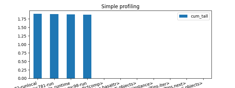
py-spy may be used to dig into native functions. An example can be found at: Profiling AdaBoostRegressor. The last piece of code uses the standard python profiler.
pr, df = profile(runlocal, as_df=True)

ax = df[['namefct', 'cum_tall']].head(n=15).set_index(
    'namefct').plot(kind='bar', figsize=(8, 3), rot=15)
ax.set_title("Simple profiling")
for la in ax.get_xticklabels():
    la.set_horizontalalignment('right')
plt.show()
Total running time of the script: ( 2 minutes 0.414 seconds)