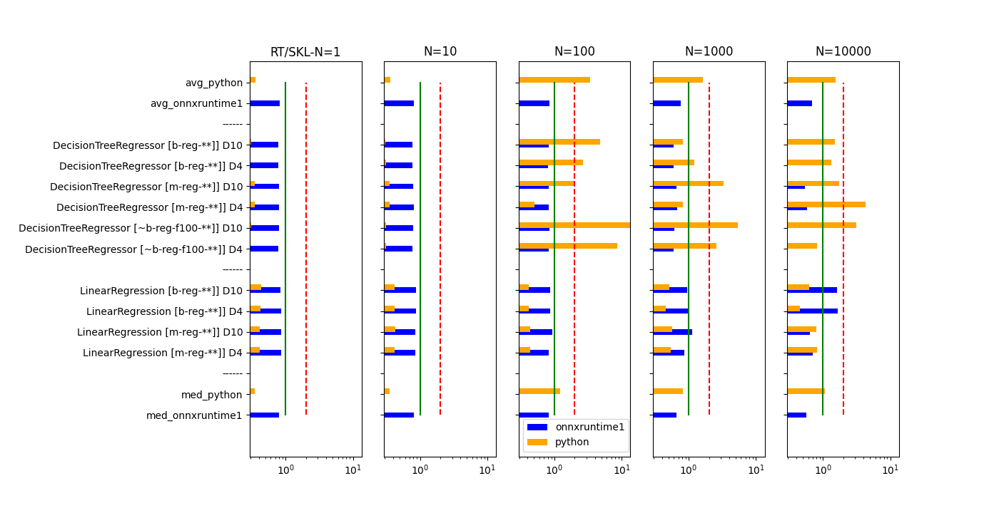
Measure ONNX runtime performances

The following example shows how to use the command line to compare one or two runtimes with scikit-learn. It relies on function validate_runtime which can be called from python or through a command line described in page Command lines.

Run the benchmark

The following line creates a folder used to dump information about models which failed during the benchmark.

import os
import matplotlib.image as mpimg
import matplotlib.pyplot as plt
import pandas
if not os.path.exists("dump_errors"):
    os.mkdir("dump_errors")

The benchmark can be run with a python instruction or a command line:

python -m mlprodict validate_runtime -v 1 --out_raw data.csv --out_summary summary.csv
           -b 1 --dump_folder dump_errors --runtime python,onnxruntime1
           --models LinearRegression,DecisionTreeRegressor
           --n_features 4,10 --out_graph bench_png
           -t "{\"1\":{\"number\":10,\"repeat\":10},\"10\":{\"number\":5,\"repeat\":5}}"

We use the python instruction in this example.

from mlprodict.cli import validate_runtime

validate_runtime(
    verbose=1,
    out_raw="data.csv", out_summary="summary.csv",
    benchmark=True, dump_folder="dump_errors",
    runtime=['python', 'onnxruntime1'],
    models=['LinearRegression', 'DecisionTreeRegressor'],
    n_features=[4, 10], dtype="32",
    out_graph="bench.png",
    time_kwargs={
        1: {"number": 100, "repeat": 100},
        10: {"number": 50, "repeat": 50},
        100: {"number": 40, "repeat": 50},
        1000: {"number": 40, "repeat": 40},
        10000: {"number": 20, "repeat": 20},
    }
)

Out:

time_kwargs={1: {'number': 100, 'repeat': 100}, 10: {'number': 50, 'repeat': 50}, 100: {'number': 40, 'repeat': 50}, 1000: {'number': 40, 'repeat': 40}, 10000: {'number': 20, 'repeat': 20}}
[enumerate_validated_operator_opsets] opset in [15, None].

  0%|          | 0/2 [00:00<?, ?it/s]
LinearRegression            :   0%|          | 0/2 [00:00<?, ?it/s][enumerate_compatible_opset] opset in [15, None].

LinearRegression            :  50%|#####     | 1/2 [04:04<04:04, 244.75s/it]
DecisionTreeRegressor       :  50%|#####     | 1/2 [04:04<04:04, 244.75s/it][enumerate_compatible_opset] opset in [15, None].

DecisionTreeRegressor       : 100%|##########| 2/2 [05:20<00:00, 145.20s/it]
DecisionTreeRegressor       : 100%|##########| 2/2 [05:20<00:00, 160.13s/it]
Saving raw_data into 'data.csv'.
Saving summary into 'summary.csv'.
Saving graph into 'bench.png'.
findfont: Font family ['STIXGeneral'] not found. Falling back to DejaVu Sans.
findfont: Font family ['STIXGeneral'] not found. Falling back to DejaVu Sans.
findfont: Font family ['STIXGeneral'] not found. Falling back to DejaVu Sans.
findfont: Font family ['STIXNonUnicode'] not found. Falling back to DejaVu Sans.
findfont: Font family ['STIXNonUnicode'] not found. Falling back to DejaVu Sans.
findfont: Font family ['STIXNonUnicode'] not found. Falling back to DejaVu Sans.
findfont: Font family ['STIXSizeOneSym'] not found. Falling back to DejaVu Sans.
findfont: Font family ['STIXSizeTwoSym'] not found. Falling back to DejaVu Sans.
findfont: Font family ['STIXSizeThreeSym'] not found. Falling back to DejaVu Sans.
findfont: Font family ['STIXSizeFourSym'] not found. Falling back to DejaVu Sans.
findfont: Font family ['STIXSizeFiveSym'] not found. Falling back to DejaVu Sans.
findfont: Font family ['cmsy10'] not found. Falling back to DejaVu Sans.
findfont: Font family ['cmr10'] not found. Falling back to DejaVu Sans.
findfont: Font family ['cmtt10'] not found. Falling back to DejaVu Sans.
findfont: Font family ['cmmi10'] not found. Falling back to DejaVu Sans.
findfont: Font family ['cmb10'] not found. Falling back to DejaVu Sans.
findfont: Font family ['cmss10'] not found. Falling back to DejaVu Sans.
findfont: Font family ['cmex10'] not found. Falling back to DejaVu Sans.
findfont: Font family ['DejaVu Sans Display'] not found. Falling back to DejaVu Sans.

Let’s show the results.

df = pandas.read_csv("summary.csv")
df.head(n=2).T

	0	1
name	DecisionTreeRegressor	DecisionTreeRegressor
problem	b-reg	b-reg
scenario	default	default
optim	NaN	NaN
method_name	predict	predict
output_index	0	0
conv_options	{}	{}
inst	{"random_state": 42}	{"random_state": 42}
n_features	4	4
runtime	onnxruntime1	python
skl_version	1.0.2	1.0.2
skl_nop	1	1
skl_ncoef	-1.0	-1.0
skl_nlin	-1.0	-1.0
skl_nnodes	223.0	223.0
skl_ntrees	1.0	1.0
skl_max_depth	13.0	13.0
onx_size	8943	8943
onx_nnodes	1	1
onx_ninits	0	0
onx_producer_name	skl2onnx	skl2onnx
onx_producer_version	1.11.1	1.11.1
onx_ai.onnx.ml	1	1
onx_size_optim	8943	8943
onx_nnodes_optim	1	1
onx_ninits_optim	0	0
opset15	OK 15/1	OK 15/1
RT/SKL-N=1	0.76977	0.302568
N=10	0.774605	0.312018
N=100	0.809891	2.637857
N=1000	0.598142	1.204685
N=10000	0.295705	1.32239
RT/SKL-N=1-min	0.647379	0.26759
RT/SKL-N=1-max	1.216684	0.308533
N=10-min	0.76104	0.306775
N=10-max	0.794946	0.319331
N=100-min	0.744827	0.354728
N=100-max	2.829383	37.263866
N=1000-min	0.578501	0.552649
N=1000-max	0.623824	11.460558
N=10000-min	0.28911	0.866072
N=10000-max	0.306857	3.55124

Let’s display the graph generated by the function.

img = mpimg.imread('bench.png')
fig = plt.imshow(img)
fig.axes.get_xaxis().set_visible(False)
fig.axes.get_yaxis().set_visible(False)
plt.show()

previous

Conversion of a logistic regression into C

next

Profile the execution of a runtime