Note
Click here to download the full example code
When to parallelize?#
That is the question. Parallize computation takes some time to set up, it is not the right solution in every case. The following example studies the parallelism introduced into the runtime of TreeEnsembleRegressor to see when it is best to do it.
from pprint import pprint
import numpy
from pandas import DataFrame
import matplotlib.pyplot as plt
from tqdm import tqdm
from sklearn import config_context
from sklearn.datasets import make_regression
from sklearn.ensemble import HistGradientBoostingRegressor
from sklearn.model_selection import train_test_split
from cpyquickhelper.numbers import measure_time
from pyquickhelper.pycode.profiling import profile
from mlprodict.onnx_conv import to_onnx, register_rewritten_operators
from mlprodict.onnxrt import OnnxInference
from mlprodict.tools.model_info import analyze_model
Available optimisations on this machine.
from mlprodict.testing.experimental_c_impl.experimental_c import code_optimisation
print(code_optimisation())
Out:
AVX-omp=8
Training and converting a model#
data = make_regression(50000, 20)
X, y = data
X_train, X_test, y_train, y_test = train_test_split(X, y)

hgb = HistGradientBoostingRegressor(max_iter=100, max_depth=6)
hgb.fit(X_train, y_train)
print(hgb)
Out:
HistGradientBoostingRegressor(max_depth=6)
Let’s get more statistics about the model itself.
pprint(analyze_model(hgb))
Out:
{'_predictors.max|tree_.max_depth': 6,
 '_predictors.size': 100,
 '_predictors.sum|tree_.leave_count': 3100,
 '_predictors.sum|tree_.node_count': 6100,
 'train_score_.shape': 101,
 'validation_score_.shape': 101}
And let’s convert it.
register_rewritten_operators()
onx = to_onnx(hgb, X_train[:1].astype(numpy.float32))
oinf = OnnxInference(onx, runtime='python_compiled')
print(oinf)
Out:
OnnxInference(...)
    def compiled_run(dict_inputs, yield_ops=None):
        if yield_ops is not None:
            raise NotImplementedError('yields_ops should be None.')
        # inputs
        X = dict_inputs['X']
        (variable, ) = n0_treeensembleregressor_1(X)
        return {
            'variable': variable,
        }
The runtime of the forest is in the following object.
print(oinf.sequence_[0].ops_)
print(oinf.sequence_[0].ops_.rt_)
Out:
TreeEnsembleRegressor_1(
    op_type=TreeEnsembleRegressor
    aggregate_function=b'SUM',
    base_values=[-0.06689953],
    base_values_as_tensor=[],
    domain=ai.onnx.ml,
    inplaces={},
    ir_version=8,
    n_targets=1,
    nodes_falsenodeids=[34 17 10 ...  0  0  0],
    nodes_featureids=[19  3  6 ...  0  0  0],
    nodes_hitrates=[1. 1. 1. ... 1. 1. 1.],
    nodes_missing_value_tracks_true=[1 0 1 ... 0 0 0],
    nodes_modes=[b'BRANCH_LEQ' b'BRANCH_LEQ' b'BRANCH_LEQ' ... b'LEAF' b'LEAF' b'LEAF'],
    nodes_nodeids=[ 0  1  2 ... 58 59 60],
    nodes_treeids=[ 0  0  0 ... 99 99 99],
    nodes_truenodeids=[1 2 3 ... 0 0 0],
    nodes_values=[ 0.08753542 -0.06473913 -0.00683493 ...  0.          0.
  0.        ],
    post_transform=b'NONE',
    runtme=None,
    target_ids=[0 0 0 ... 0 0 0],
    target_nodeids=[ 5  6  8 ... 58 59 60],
    target_opset=1,
    target_treeids=[ 0  0  0 ... 99 99 99],
    target_weights=[-33.69531    -22.34756    -21.788332   ...   0.74944806   2.0057945
   2.1422892 ],
)
<mlprodict.onnxrt.ops_cpu.op_tree_ensemble_regressor_p_.RuntimeTreeEnsembleRegressorPFloat object at 0x7f434ee93870>
And the threshold used to start parallelizing based on the number of observations.
print(oinf.sequence_[0].ops_.rt_.omp_N_)
Out:
20
Profiling#
This step involves pyinstrument to measure where the time is spent. Both scikit-learn and mlprodict runtime are called so that the prediction times can be compared.
X32 = X_test.astype(numpy.float32)


def runlocal():
    with config_context(assume_finite=True):
        for i in range(0, 100):
            oinf.run({'X': X32[:1000]})
            hgb.predict(X_test[:1000])


print("profiling...")
txt = profile(runlocal, pyinst_format='text')
print(txt[1])
Out:
profiling...

  _     ._   __/__   _ _  _  _ _/_   Recorded: 04:28:21 AM Samples:  7255
 /_//_/// /_\ / //_// / //_'/ //     Duration: 113.898   CPU time: 787.190
/   _/                      v4.1.1

Program: /var/lib/jenkins/workspace/mlprodict/mlprodict_UT_39_std/_doc/examples/plot_parallelism.py

113.898 profile  ../pycode/profiling.py:457
`- 113.898 runlocal  plot_parallelism.py:91
      [35 frames hidden]  plot_parallelism, sklearn, <built-in>...
         112.215 _predict_from_raw_data  <built-in>:0
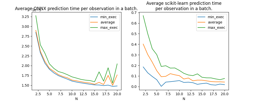
Now let’s measure the performance the average computation time per observations for 2 to 100 observations. The runtime implemented in mlprodict parallizes the computation after a given number of observations.
obs = []
for N in tqdm(list(range(2, 21))):
    m = measure_time("oinf.run({'X': x})",
                     {'oinf': oinf, 'x': X32[:N]},
                     div_by_number=True,
                     number=20)
    m['N'] = N
    m['RT'] = 'ONNX'
    obs.append(m)

    with config_context(assume_finite=True):
        m = measure_time("hgb.predict(x)",
                         {'hgb': hgb, 'x': X32[:N]},
                         div_by_number=True,
                         number=15)
    m['N'] = N
    m['RT'] = 'SKL'
    obs.append(m)

df = DataFrame(obs)
num = ['min_exec', 'average', 'max_exec']
for c in num:
    df[c] /= df['N']
df.head()
Out:
  0%|          | 0/19 [00:00<?, ?it/s]
  5%|5         | 1/19 [02:00<36:11, 120.61s/it]
 11%|#         | 2/19 [04:17<36:50, 130.02s/it]
 16%|#5        | 3/19 [06:35<35:44, 134.01s/it]
 21%|##1       | 4/19 [08:28<31:22, 125.51s/it]
 26%|##6       | 5/19 [09:52<25:46, 110.48s/it]
 32%|###1      | 6/19 [11:33<23:17, 107.49s/it]
 37%|###6      | 7/19 [14:00<24:02, 120.20s/it]
 42%|####2     | 8/19 [16:30<23:46, 129.67s/it]
 47%|####7     | 9/19 [19:04<22:54, 137.47s/it]
 53%|#####2    | 10/19 [21:02<19:42, 131.42s/it]
 58%|#####7    | 11/19 [23:28<18:06, 135.75s/it]
 63%|######3   | 12/19 [25:14<14:47, 126.85s/it]
 68%|######8   | 13/19 [27:22<12:42, 127.08s/it]
 74%|#######3  | 14/19 [29:38<10:48, 129.75s/it]
 79%|#######8  | 15/19 [31:48<08:39, 129.96s/it]
 84%|########4 | 16/19 [33:50<06:22, 127.35s/it]
 89%|########9 | 17/19 [35:50<04:10, 125.37s/it]
 95%|#########4| 18/19 [37:58<02:06, 126.07s/it]
100%|##########| 19/19 [40:06<00:00, 126.69s/it]
100%|##########| 19/19 [40:06<00:00, 126.67s/it]
Graph.
fig, ax = plt.subplots(1, 2, figsize=(10, 4))
df[df.RT == 'ONNX'].set_index('N')[num].plot(ax=ax[0])
ax[0].set_title("Average ONNX prediction time per observation in a batch.")
df[df.RT == 'SKL'].set_index('N')[num].plot(ax=ax[1])
ax[1].set_title(
    "Average scikit-learn prediction time\nper observation in a batch.")
Out:
Text(0.5, 1.0, 'Average scikit-learn prediction time\nper observation in a batch.')
Gain from parallelization#
There is a clear gap between after and before 10 observations when it is parallelized. Does this threshold depends on the number of trees in the model? For that we compute for each model the average prediction time up to 10 and from 10 to 20.
def parallized_gain(df):
    df = df[df.RT == 'ONNX']
    df10 = df[df.N <= 10]
    t10 = sum(df10['average']) / df10.shape[0]
    df10p = df[df.N > 10]
    t10p = sum(df10p['average']) / df10p.shape[0]
    return t10 / t10p


print('gain', parallized_gain(df))
Out:
gain 1.2512508977515335
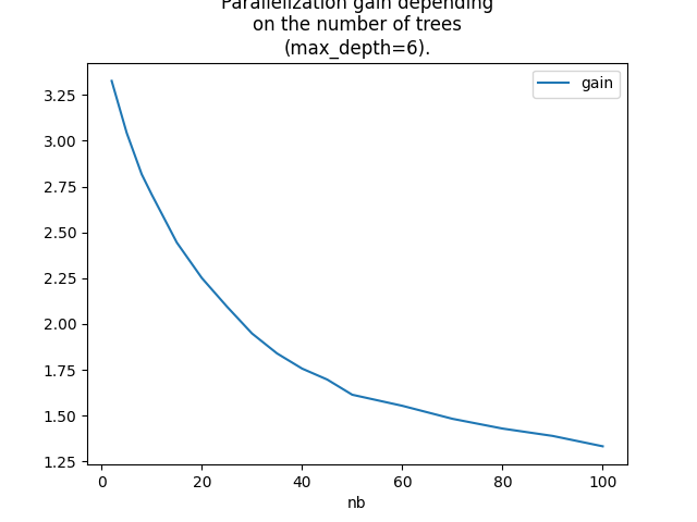
Measures based on the number of trees#
We trained many models with different number of trees to see how the parallelization gain is moving. One models is trained for every distinct number of trees and then the prediction time is measured for different number of observations.
tries_set = [2, 5, 8] + list(range(10, 50, 5)) + list(range(50, 101, 10))
tries = [(nb, N) for N in range(2, 21, 2) for nb in tries_set]
training
models = {100: (hgb, oinf)}
for nb in tqdm(set(_[0] for _ in tries)):
    if nb not in models:
        hgb = HistGradientBoostingRegressor(max_iter=nb, max_depth=6)
        hgb.fit(X_train, y_train)
        onx = to_onnx(hgb, X_train[:1].astype(numpy.float32))
        oinf = OnnxInference(onx, runtime='python_compiled')
        models[nb] = (hgb, oinf)
Out:
  0%|          | 0/17 [00:00<?, ?it/s]
  6%|5         | 1/17 [00:05<01:31,  5.74s/it]
 12%|#1        | 2/17 [00:43<06:09, 24.61s/it]
 24%|##3       | 4/17 [00:49<02:23, 11.04s/it]
 29%|##9       | 5/17 [02:18<07:00, 35.06s/it]
 35%|###5      | 6/17 [02:31<05:13, 28.48s/it]
 41%|####1     | 7/17 [03:20<05:46, 34.64s/it]
 47%|####7     | 8/17 [03:31<04:07, 27.53s/it]
 53%|#####2    | 9/17 [04:20<04:31, 33.99s/it]
 59%|#####8    | 10/17 [04:49<03:46, 32.36s/it]
 65%|######4   | 11/17 [07:07<06:25, 64.32s/it]
 71%|#######   | 12/17 [08:03<05:09, 61.81s/it]
 76%|#######6  | 13/17 [08:27<03:21, 50.44s/it]
 82%|########2 | 14/17 [08:53<02:09, 43.08s/it]
 88%|########8 | 15/17 [11:15<02:25, 72.64s/it]
 94%|#########4| 16/17 [12:52<01:20, 80.09s/it]
100%|##########| 17/17 [13:38<00:00, 69.87s/it]
100%|##########| 17/17 [13:38<00:00, 48.15s/it]
prediction time
obs = []

for nb, N in tqdm(tries):
    hgb, oinf = models[nb]
    m = measure_time("oinf.run({'X': x})",
                     {'oinf': oinf, 'x': X32[:N]},
                     div_by_number=True,
                     number=50)
    m['N'] = N
    m['nb'] = nb
    m['RT'] = 'ONNX'
    obs.append(m)

df = DataFrame(obs)
num = ['min_exec', 'average', 'max_exec']
for c in num:
    df[c] /= df['N']
df.head()
Out:
  0%|          | 0/170 [00:00<?, ?it/s]
  4%|3         | 6/170 [00:00<00:02, 57.38it/s]
  7%|7         | 12/170 [00:00<00:03, 50.62it/s]
 11%|#         | 18/170 [00:00<00:03, 44.81it/s]
 14%|#4        | 24/170 [00:00<00:03, 47.06it/s]
 17%|#7        | 29/170 [00:00<00:03, 43.62it/s]
 20%|##        | 34/170 [00:00<00:03, 36.60it/s]
 24%|##3       | 40/170 [00:00<00:03, 40.54it/s]
 26%|##6       | 45/170 [00:01<00:03, 38.41it/s]
 29%|##8       | 49/170 [00:01<00:03, 33.60it/s]
 31%|###1      | 53/170 [00:01<00:03, 31.88it/s]
 34%|###4      | 58/170 [00:01<00:03, 34.76it/s]
 36%|###6      | 62/170 [00:01<00:03, 32.84it/s]
 39%|###8      | 66/170 [00:01<00:03, 28.11it/s]
 41%|####      | 69/170 [00:01<00:03, 25.69it/s]
 44%|####3     | 74/170 [00:02<00:03, 30.20it/s]
 46%|####5     | 78/170 [00:02<00:03, 29.51it/s]
 48%|####8     | 82/170 [00:02<00:03, 25.68it/s]
 50%|#####     | 85/170 [00:02<00:04, 21.12it/s]
 53%|#####2    | 90/170 [00:02<00:03, 26.38it/s]
 55%|#####5    | 94/170 [00:02<00:02, 26.90it/s]
 57%|#####7    | 97/170 [00:03<00:02, 24.92it/s]
 59%|#####8    | 100/170 [00:03<00:03, 21.16it/s]
 61%|######    | 103/170 [00:03<00:03, 19.11it/s]
 64%|######3   | 108/170 [00:03<00:02, 23.98it/s]
 65%|######5   | 111/170 [00:03<00:02, 24.06it/s]
 67%|######7   | 114/170 [00:03<00:02, 22.16it/s]
 69%|######8   | 117/170 [00:04<00:02, 18.56it/s]
 71%|#######   | 120/170 [00:04<00:02, 16.75it/s]
 74%|#######3  | 125/170 [00:04<00:02, 21.63it/s]
 75%|#######5  | 128/170 [00:04<00:01, 21.84it/s]
 77%|#######7  | 131/170 [00:04<00:01, 20.11it/s]
 79%|#######8  | 134/170 [00:05<00:02, 16.75it/s]
 80%|########  | 136/170 [00:05<00:02, 14.01it/s]
 83%|########2 | 141/170 [00:05<00:01, 19.59it/s]
 85%|########4 | 144/170 [00:05<00:01, 20.58it/s]
 86%|########6 | 147/170 [00:05<00:01, 19.33it/s]
 88%|########8 | 150/170 [00:05<00:01, 16.47it/s]
 89%|########9 | 152/170 [00:06<00:01, 13.92it/s]
 91%|######### | 154/170 [00:06<00:01, 13.68it/s]
 93%|#########2| 158/170 [00:06<00:00, 18.41it/s]
 95%|#########4| 161/170 [00:06<00:00, 19.44it/s]
 96%|#########6| 164/170 [00:06<00:00, 18.03it/s]
 98%|#########8| 167/170 [00:07<00:00, 15.00it/s]
 99%|#########9| 169/170 [00:07<00:00, 12.60it/s]
100%|##########| 170/170 [00:07<00:00, 22.83it/s]
Let’s compute the gains.
gains = []
for nb in set(df['nb']):
    gain = parallized_gain(df[df.nb == nb])
    gains.append(dict(nb=nb, gain=gain))

dfg = DataFrame(gains)
dfg = dfg.sort_values('nb').reset_index(drop=True).copy()
dfg
Graph.
ax = dfg.set_index('nb').plot()
ax.set_title(
    "Parallelization gain depending\non the number of trees\n(max_depth=6).")
Out:
Text(0.5, 1.0, 'Parallelization gain depending\non the number of trees\n(max_depth=6).')
That does not answer the question we are looking for
as we would like to know the best threshold th
which defines the number of observations for which
we should parallelized. This number depends on the number
of trees. A gain > 1 means the parallization should happen
Here, even two observations is ok.
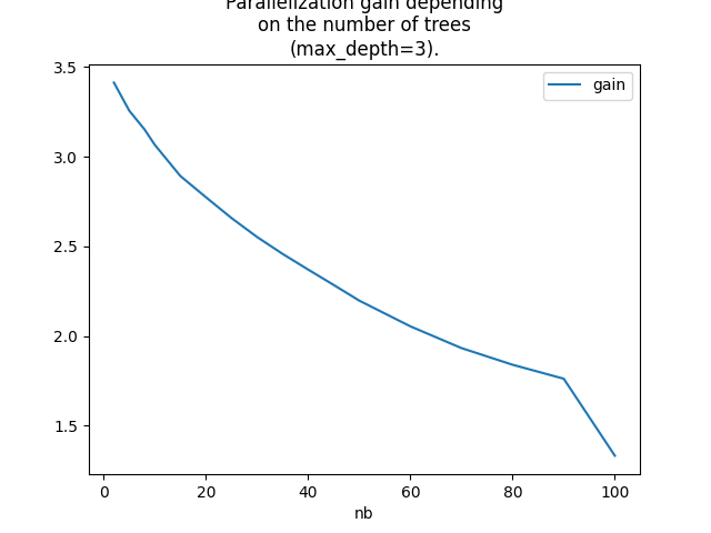
Let’s check with lighter trees (max_depth=2),
maybe in that case, the conclusion is different.
models = {100: (hgb, oinf)}
for nb in tqdm(set(_[0] for _ in tries)):
    if nb not in models:
        hgb = HistGradientBoostingRegressor(max_iter=nb, max_depth=2)
        hgb.fit(X_train, y_train)
        onx = to_onnx(hgb, X_train[:1].astype(numpy.float32))
        oinf = OnnxInference(onx, runtime='python_compiled')
        models[nb] = (hgb, oinf)

obs = []
for nb, N in tqdm(tries):
    hgb, oinf = models[nb]
    m = measure_time("oinf.run({'X': x})",
                     {'oinf': oinf, 'x': X32[:N]},
                     div_by_number=True,
                     number=50)
    m['N'] = N
    m['nb'] = nb
    m['RT'] = 'ONNX'
    obs.append(m)

df = DataFrame(obs)
num = ['min_exec', 'average', 'max_exec']
for c in num:
    df[c] /= df['N']
df.head()
Out:
  0%|          | 0/17 [00:00<?, ?it/s]
  6%|5         | 1/17 [00:01<00:21,  1.34s/it]
 12%|#1        | 2/17 [00:11<01:38,  6.53s/it]
 24%|##3       | 4/17 [00:12<00:36,  2.77s/it]
 29%|##9       | 5/17 [00:26<01:15,  6.31s/it]
 35%|###5      | 6/17 [00:28<00:55,  5.05s/it]
 41%|####1     | 7/17 [00:36<00:58,  5.84s/it]
 47%|####7     | 8/17 [00:39<00:43,  4.86s/it]
 53%|#####2    | 9/17 [00:48<00:50,  6.30s/it]
 59%|#####8    | 10/17 [00:52<00:37,  5.35s/it]
 65%|######4   | 11/17 [01:13<01:00, 10.17s/it]
 71%|#######   | 12/17 [01:28<00:58, 11.69s/it]
 76%|#######6  | 13/17 [01:33<00:38,  9.65s/it]
 82%|########2 | 14/17 [01:38<00:24,  8.19s/it]
 88%|########8 | 15/17 [02:01<00:25, 12.79s/it]
 94%|#########4| 16/17 [02:15<00:13, 13.15s/it]
100%|##########| 17/17 [02:24<00:00, 11.70s/it]
100%|##########| 17/17 [02:24<00:00,  8.48s/it]

  0%|          | 0/170 [00:00<?, ?it/s]
  4%|4         | 7/170 [00:00<00:02, 59.61it/s]
  8%|7         | 13/170 [00:00<00:02, 56.36it/s]
 11%|#1        | 19/170 [00:00<00:02, 52.42it/s]
 15%|#4        | 25/170 [00:00<00:02, 53.54it/s]
 18%|#8        | 31/170 [00:00<00:02, 51.02it/s]
 22%|##1       | 37/170 [00:00<00:02, 47.34it/s]
 25%|##5       | 43/170 [00:00<00:02, 48.47it/s]
 28%|##8       | 48/170 [00:00<00:02, 46.28it/s]
 31%|###1      | 53/170 [00:01<00:02, 41.70it/s]
 35%|###4      | 59/170 [00:01<00:02, 44.30it/s]
 38%|###7      | 64/170 [00:01<00:02, 43.00it/s]
 41%|####      | 69/170 [00:01<00:02, 36.76it/s]
 44%|####4     | 75/170 [00:01<00:02, 40.56it/s]
 47%|####7     | 80/170 [00:01<00:02, 40.19it/s]
 50%|#####     | 85/170 [00:02<00:02, 32.70it/s]
 54%|#####3    | 91/170 [00:02<00:02, 37.33it/s]
 56%|#####6    | 96/170 [00:02<00:01, 37.73it/s]
 59%|#####9    | 101/170 [00:02<00:02, 33.83it/s]
 62%|######1   | 105/170 [00:02<00:02, 31.75it/s]
 65%|######4   | 110/170 [00:02<00:01, 34.74it/s]
 67%|######7   | 114/170 [00:02<00:01, 34.43it/s]
 69%|######9   | 118/170 [00:03<00:01, 30.53it/s]
 72%|#######1  | 122/170 [00:03<00:01, 28.55it/s]
 75%|#######4  | 127/170 [00:03<00:01, 32.04it/s]
 77%|#######7  | 131/170 [00:03<00:01, 31.92it/s]
 79%|#######9  | 135/170 [00:03<00:01, 28.09it/s]
 81%|########1 | 138/170 [00:03<00:01, 25.24it/s]
 84%|########4 | 143/170 [00:03<00:00, 29.81it/s]
 86%|########6 | 147/170 [00:03<00:00, 30.41it/s]
 89%|########8 | 151/170 [00:04<00:00, 27.48it/s]
 91%|######### | 154/170 [00:04<00:00, 22.45it/s]
 94%|#########3| 159/170 [00:04<00:00, 27.62it/s]
 96%|#########5| 163/170 [00:04<00:00, 28.91it/s]
 98%|#########8| 167/170 [00:04<00:00, 27.01it/s]
100%|##########| 170/170 [00:05<00:00, 20.09it/s]
100%|##########| 170/170 [00:05<00:00, 33.63it/s]
Measures.
gains = []
for nb in set(df['nb']):
    gain = parallized_gain(df[df.nb == nb])
    gains.append(dict(nb=nb, gain=gain))

dfg = DataFrame(gains)
dfg = dfg.sort_values('nb').reset_index(drop=True).copy()
dfg
Graph.
ax = dfg.set_index('nb').plot()
ax.set_title(
    "Parallelization gain depending\non the number of trees\n(max_depth=3).")
Out:
Text(0.5, 1.0, 'Parallelization gain depending\non the number of trees\n(max_depth=3).')
The conclusion is somewhat the same but it shows that the bigger the number of trees is the bigger the gain is and under the number of cores of the processor.
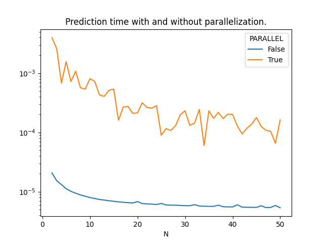
Moving the theshold#
The last experiment consists in comparing the prediction time with or without parallelization for different number of observation.
hgb = HistGradientBoostingRegressor(max_iter=40, max_depth=6)
hgb.fit(X_train, y_train)
onx = to_onnx(hgb, X_train[:1].astype(numpy.float32))
oinf = OnnxInference(onx, runtime='python_compiled')


obs = []
for N in tqdm(list(range(2, 51))):
    oinf.sequence_[0].ops_.rt_.omp_N_ = 100
    m = measure_time("oinf.run({'X': x})",
                     {'oinf': oinf, 'x': X32[:N]},
                     div_by_number=True,
                     number=20)
    m['N'] = N
    m['RT'] = 'ONNX'
    m['PARALLEL'] = False
    obs.append(m)

    oinf.sequence_[0].ops_.rt_.omp_N_ = 1
    m = measure_time("oinf.run({'X': x})",
                     {'oinf': oinf, 'x': X32[:N]},
                     div_by_number=True,
                     number=50)
    m['N'] = N
    m['RT'] = 'ONNX'
    m['PARALLEL'] = True
    obs.append(m)

df = DataFrame(obs)
num = ['min_exec', 'average', 'max_exec']
for c in num:
    df[c] /= df['N']
df.head()
Out:
  0%|          | 0/49 [00:00<?, ?it/s]
  2%|2         | 1/49 [00:03<03:11,  4.00s/it]
  4%|4         | 2/49 [00:07<03:06,  3.97s/it]
  6%|6         | 3/49 [00:09<02:08,  2.79s/it]
  8%|8         | 4/49 [00:13<02:25,  3.24s/it]
 10%|#         | 5/49 [00:15<02:05,  2.86s/it]
 12%|#2        | 6/49 [00:19<02:16,  3.18s/it]
 14%|#4        | 7/49 [00:21<02:01,  2.89s/it]
 16%|#6        | 8/49 [00:23<01:52,  2.75s/it]
 18%|#8        | 9/49 [00:28<02:06,  3.16s/it]
 20%|##        | 10/49 [00:32<02:13,  3.43s/it]
 22%|##2       | 11/49 [00:34<02:00,  3.18s/it]
 24%|##4       | 12/49 [00:37<01:51,  3.02s/it]
 27%|##6       | 13/49 [00:41<01:55,  3.21s/it]
 29%|##8       | 14/49 [00:45<02:01,  3.47s/it]
 31%|###       | 15/49 [00:46<01:35,  2.82s/it]
 33%|###2      | 16/49 [00:48<01:27,  2.66s/it]
 35%|###4      | 17/49 [00:51<01:23,  2.62s/it]
 37%|###6      | 18/49 [00:53<01:15,  2.44s/it]
 39%|###8      | 19/49 [00:55<01:10,  2.36s/it]
 41%|####      | 20/49 [00:58<01:17,  2.66s/it]
 43%|####2     | 21/49 [01:01<01:16,  2.74s/it]
 45%|####4     | 22/49 [01:04<01:15,  2.81s/it]
 47%|####6     | 23/49 [01:08<01:18,  3.00s/it]
 49%|####8     | 24/49 [01:09<01:01,  2.45s/it]
 51%|#####1    | 25/49 [01:10<00:52,  2.18s/it]
 53%|#####3    | 26/49 [01:12<00:45,  1.97s/it]
 55%|#####5    | 27/49 [01:14<00:42,  1.94s/it]
 57%|#####7    | 28/49 [01:17<00:46,  2.23s/it]
 59%|#####9    | 29/49 [01:20<00:52,  2.62s/it]
 61%|######1   | 30/49 [01:22<00:46,  2.46s/it]
 63%|######3   | 31/49 [01:25<00:43,  2.42s/it]
 65%|######5   | 32/49 [01:29<00:49,  2.92s/it]
 67%|######7   | 33/49 [01:30<00:37,  2.36s/it]
 69%|######9   | 34/49 [01:34<00:43,  2.88s/it]
 71%|#######1  | 35/49 [01:37<00:41,  2.97s/it]
 73%|#######3  | 36/49 [01:41<00:42,  3.30s/it]
 76%|#######5  | 37/49 [01:44<00:39,  3.31s/it]
 78%|#######7  | 38/49 [01:48<00:38,  3.52s/it]
 80%|#######9  | 39/49 [01:52<00:36,  3.69s/it]
 82%|########1 | 40/49 [01:55<00:30,  3.38s/it]
 84%|########3 | 41/49 [01:57<00:23,  2.98s/it]
 86%|########5 | 42/49 [02:00<00:20,  2.86s/it]
 88%|########7 | 43/49 [02:03<00:17,  2.93s/it]
 90%|########9 | 44/49 [02:07<00:16,  3.27s/it]
 92%|#########1| 45/49 [02:10<00:12,  3.18s/it]
 94%|#########3| 46/49 [02:12<00:09,  3.01s/it]
 96%|#########5| 47/49 [02:15<00:05,  2.88s/it]
 98%|#########7| 48/49 [02:17<00:02,  2.51s/it]
100%|##########| 49/49 [02:21<00:00,  3.00s/it]
100%|##########| 49/49 [02:21<00:00,  2.88s/it]
Graph.
piv = df[['N', 'PARALLEL', 'average']].pivot('N', 'PARALLEL', 'average')
ax = piv.plot(logy=True)
ax.set_title("Prediction time with and without parallelization.")
Out:
Text(0.5, 1.0, 'Prediction time with and without parallelization.')
Parallelization is working.
plt.show()
Total running time of the script: ( 64 minutes 20.979 seconds)