Note
Click here to download the full example code
TopK benchmark#
This example compares onnxruntime and mlprodict for an implementation of operator TopK. We measure two runtimes by computing a ratio between their time execution through the following kind of graphs.
Graph to compare performance#
from numpy.random import randn
import numpy
import matplotlib.pyplot as plt
from pandas import DataFrame
from onnxruntime import InferenceSession, __version__ as ort_version
from tqdm import tqdm
from cpyquickhelper.numbers import measure_time
from pyquickhelper.pycode.profiling import profile
from skl2onnx.algebra.onnx_ops import OnnxTopK_11
from skl2onnx.common.data_types import FloatTensorType
from skl2onnx.algebra.onnx_ops import OnnxTopK
from mlprodict.onnxrt.validate.validate_benchmark import benchmark_fct
from mlprodict.onnxrt import OnnxInference
from mlprodict.onnxrt.ops_cpu.op_topk import (
    topk_sorted_implementation, topk_sorted_implementation_cpp)
from mlprodict import __version__ as mlp_version
from mlprodict.plotting.plotting import plot_benchmark_metrics
Available optimisation on this machine.
from mlprodict.testing.experimental_c_impl.experimental_c import code_optimisation
print(code_optimisation())
Out:
AVX-omp=8
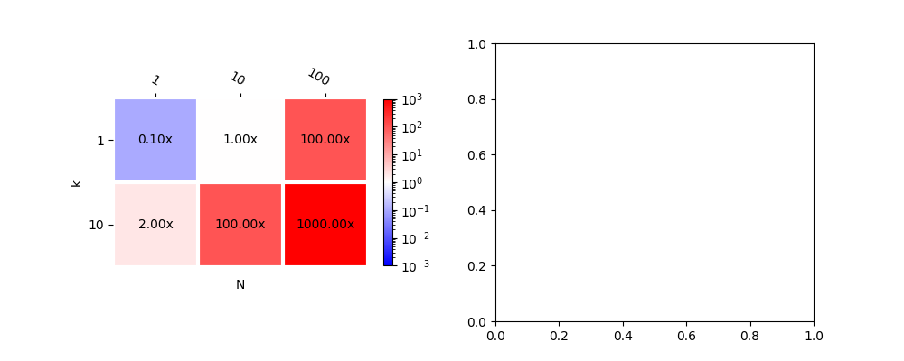
Graph.
def plot_metric(metric, ax=None, xlabel="N", ylabel="k", middle=1.,
                transpose=False, shrink=1.0, title=None):
    ax, cbar = plot_benchmark_metrics(
        metric, ax=ax, xlabel=xlabel, ylabel=ylabel, middle=middle,
        transpose=transpose, cbar_kw={'shrink': shrink})
    if title is not None:
        ax.set_title(title)
    return ax


data = {(1, 1): 0.1, (10, 1): 1, (1, 10): 2,
        (10, 10): 100, (100, 1): 100, (100, 10): 1000}

fig, ax = plt.subplots(1, 2, figsize=(10, 4))
plot_metric(data, ax[0], shrink=0.6)
Out:
<AxesSubplot:xlabel='N', ylabel='k'>
plot_metric(data, ax[1], transpose=True)
Out:
<AxesSubplot:xlabel='k', ylabel='N'>
TopK in ONNX#
The following lines creates an ONNX graph using one TopK ONNX node. The outcome is the ONNX graph converted into json.
X32 = randn(100000, 100).astype(numpy.float32)

node = OnnxTopK_11('X', numpy.array([5], dtype=numpy.int64),
                   output_names=['dist', 'ind'])

model_onnx = node.to_onnx(
    [('X', X32)], target_opset=12,
    # shape inference does not seem to work in onnxruntime
    # so we speccify the output shape
    outputs=[('dist', X32[:1, :5]),
             ('ind', X32[:1, :5].astype(numpy.int64))])
model_onnx
Out:
ir_version: 6
producer_name: "skl2onnx"
producer_version: "1.11.1"
domain: "ai.onnx"
model_version: 0
graph {
  node {
    input: "X"
    input: "To_TopKcst"
    output: "dist"
    output: "ind"
    name: "To_TopK"
    op_type: "TopK"
    domain: ""
  }
  name: "OnnxTopK_11"
  initializer {
    dims: 1
    data_type: 7
    int64_data: 5
    name: "To_TopKcst"
  }
  input {
    name: "X"
    type {
      tensor_type {
        elem_type: 1
        shape {
          dim {
          }
          dim {
            dim_value: 100
          }
        }
      }
    }
  }
  output {
    name: "dist"
    type {
      tensor_type {
        elem_type: 1
        shape {
          dim {
          }
          dim {
            dim_value: 5
          }
        }
      }
    }
  }
  output {
    name: "ind"
    type {
      tensor_type {
        elem_type: 7
        shape {
          dim {
          }
          dim {
            dim_value: 5
          }
        }
      }
    }
  }
}
opset_import {
  domain: ""
  version: 11
}
That gives…
oinf = OnnxInference(model_onnx, runtime="python")
res = oinf.run({'X': X32})
dist, ind = res['dist'], res['ind']
dist[:2], ind[:2]
Out:
(array([[2.0272512, 1.8558152, 1.8149445, 1.4867951, 1.3442959],
       [2.6460865, 1.7889596, 1.7093822, 1.4970592, 1.4434265]],
      dtype=float32), array([[64, 77,  9, 61, 47],
       [ 9, 25, 36, 44,  6]]))
With onnxruntime.
sess = InferenceSession(model_onnx.SerializeToString())
dist, ind = sess.run(None, {'X': X32})
dist[:2], ind[:2]
Out:
(array([[2.0272512, 1.8558152, 1.8149445, 1.4867951, 1.3442959],
       [2.6460865, 1.7889596, 1.7093822, 1.4970592, 1.4434265]],
      dtype=float32), array([[64, 77,  9, 61, 47],
       [ 9, 25, 36, 44,  6]], dtype=int64))
Let’s compare two implementations.
def benchmark(X, fct1, fct2, N, repeat=10, number=10):

    def ti(n):
        if n <= 1:
            return 50
        if n <= 1000:
            return 2
        if n <= 10000:
            return 0.51
        return 0.11

    # to warm up the engine
    time_kwargs = {n: dict(repeat=10, number=10) for n in N[:2]}
    benchmark_fct(fct1, X, time_kwargs=time_kwargs, skip_long_test=False)
    benchmark_fct(fct2, X, time_kwargs=time_kwargs, skip_long_test=False)
    # real measure
    time_kwargs = {n: dict(repeat=int(repeat * ti(n)),
                           number=int(number * ti(n))) for n in N}
    res1 = benchmark_fct(fct1, X, time_kwargs=time_kwargs,
                         skip_long_test=False)
    res2 = benchmark_fct(fct2, X, time_kwargs=time_kwargs,
                         skip_long_test=False)

    res = {}
    for r in sorted(res1):
        r1 = res1[r]
        r2 = res2[r]
        ratio = r2['ttime'] / r1['ttime']
        res[r] = ratio
    return res


N = [1, 10, 100, 1000, 10000, 100000]
res = benchmark(X32, lambda x: sess.run(None, {'X': x}),
                lambda x: oinf.run({'X': x}), N=N)
res
Out:
{1: 1.3491936839804246, 10: 1.2996703310122397, 100: 24.31770123598381, 1000: 11.200222562568541, 10000: 2.680006426590349, 100000: 1.0835793513909697}
The implementation in mlprodict is faster when the number of rows grows. It is faster for 1 rows, for many rows, the implementation uses openmp to parallelize.
C++ implementation vs numpy#
scikit-learn uses numpy to compute the top k elements.
res = benchmark(X32, lambda x: topk_sorted_implementation(x, 5, 1, 0),
                lambda x: topk_sorted_implementation_cpp(x, 5, 1, 0), N=N)
res
Out:
{1: 0.3050468267705555, 10: 0.29974319199162397, 100: 8.586906612338494, 1000: 1.8539561753429743, 10000: 0.3519928839345043, 100000: 0.13709498200454023}
It seems to be faster too. Let’s profile.
xr = randn(1000000, 100)
text = profile(lambda: topk_sorted_implementation(xr, 5, 1, 0),
               pyinst_format='text')[1]
print(text)
Out:
  _     ._   __/__   _ _  _  _ _/_   Recorded: 05:48:31 AM Samples:  5
 /_//_/// /_\ / //_// / //_'/ //     Duration: 6.664     CPU time: 6.599
/   _/                      v4.1.1

Program: /var/lib/jenkins/workspace/mlprodict/mlprodict_UT_39_std/_doc/examples/plot_op_onnx_topk.py

6.664 profile  ../pycode/profiling.py:457
`- 6.664 <lambda>  plot_op_onnx_topk.py:177
      [15 frames hidden]  plot_op_onnx_topk, mlprodict, <__arra...
         5.336 ndarray.argpartition  <built-in>:0
Parallelisation#
We need to disable the parallelisation to really compare both implementation.
# In[11]:


def benchmark_test(X, fct1, fct2, N, K, repeat=10, number=10):
    res = {}
    for k in tqdm(K):
        def f1(x, k=k): return fct1(x, k=k)
        def f2(x, k=k): return fct2(x, k=k)
        r = benchmark(X32, f1, f2, N=N, repeat=repeat, number=number)
        for n, v in r.items():
            res[n, k] = v
    return res


K = [1, 2, 5, 10, 15]
N = [1, 2, 3, 10, 100, 1000, 10000]

bench_para = benchmark_test(
    X32, (lambda x, k: topk_sorted_implementation_cpp(
        x, k=k, axis=1, largest=0, th_para=100000000)),
    (lambda x, k: topk_sorted_implementation_cpp(
        x, k=k, axis=1, largest=0, th_para=1)),
    N=N, K=K)

bench_para
Out:
  0%|          | 0/5 [00:00<?, ?it/s]
 20%|##        | 1/5 [00:29<01:56, 29.22s/it]
 40%|####      | 2/5 [01:02<01:34, 31.46s/it]
 60%|######    | 3/5 [01:35<01:04, 32.47s/it]
 80%|########  | 4/5 [02:06<00:31, 31.87s/it]
100%|##########| 5/5 [02:40<00:00, 32.36s/it]
100%|##########| 5/5 [02:40<00:00, 32.02s/it]

{(1, 1): 1.0019932270429421, (2, 1): 220.80063479781504, (3, 1): 221.67549421569402, (10, 1): 69.233887837786, (100, 1): 24.453764003632923, (1000, 1): 20.776148018831723, (10000, 1): 2.5208520860435053, (1, 2): 0.9953727637513775, (2, 2): 72.22934386606052, (3, 2): 220.9212633588702, (10, 2): 194.68582938198458, (100, 2): 82.42947243987165, (1000, 2): 12.475049139663017, (10000, 2): 1.4807891809287688, (1, 5): 0.9976739836905998, (2, 5): 215.0298508146255, (3, 5): 93.43249284395424, (10, 5): 158.9577147990169, (100, 5): 48.49672393457181, (1000, 5): 5.738895557417205, (10000, 5): 0.8801927954561015, (1, 10): 0.9968480030454562, (2, 10): 106.72026978546145, (3, 10): 100.2405380008792, (10, 10): 47.303245103046756, (100, 10): 23.654833569670085, (1000, 10): 2.610032781828763, (10000, 10): 0.5377695979668052, (1, 15): 0.9952193911710505, (2, 15): 113.64538418489951, (3, 15): 68.265585458802, (10, 15): 111.67960543582143, (100, 15): 8.761230393816833, (1000, 15): 2.300441861980231, (10000, 15): 0.44169301848551096}
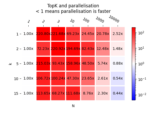
As a graph.
plot_metric(bench_para, transpose=False, title="TopK and parallelisation\n"
            "< 1 means parallelisation is faster", shrink=0.75)
Out:
<AxesSubplot:title={'center':'TopK and parallelisation\n< 1 means parallelisation is faster'}, xlabel='N', ylabel='k'>
This is somehow expected. First column is closed to 1 as it is the same code being compared. Next columns are red, meaning the parallelisation does not help, the parallelisation helps for bigger N, as least more than 100.
Parallellisation with ONNX#
We replicate the same experiment with an ONNX graph.
k_ = numpy.array([3], dtype=numpy.int64)
node = OnnxTopK_11('X', 'k',
                   output_names=['dist', 'ind'])

model_onnx = node.to_onnx(
    [('X', X32), ('k', k_)], target_opset=12,
    # shape inference does not seem to work in onnxruntime
    # so we speccify the output shape
    outputs=[('dist', X32[:1, :5]),
             ('ind', X32[:1, :5].astype(numpy.int64))])
Test
oinf_no_para = OnnxInference(model_onnx, runtime="python")
res = oinf_no_para.run({'X': X32, 'k': k_})
dist, ind = res['dist'], res['ind']
dist[:2], ind[:2]
Out:
(array([[2.0272512, 1.8558152, 1.8149445],
       [2.6460865, 1.7889596, 1.7093822]], dtype=float32), array([[64, 77,  9],
       [ 9, 25, 36]]))
Let’s play with the thresholds triggering the parallelisation.
oinf_para = OnnxInference(model_onnx, runtime="python")
oinf_no_para.sequence_[0].ops_.th_para = 100000000
oinf_para.sequence_[0].ops_.th_para = 1
Results.
bench_onnx_para = benchmark_test(
    X32, (lambda x, k: oinf_no_para.run(
        {'X': x, 'k': numpy.array([k], dtype=numpy.int64)})),
    (lambda x, k: oinf_para.run(
        {'X': x, 'k': numpy.array([k], dtype=numpy.int64)})),
    N=N, K=K)
bench_onnx_para
Out:
  0%|          | 0/5 [00:00<?, ?it/s]
 20%|##        | 1/5 [01:05<04:23, 65.95s/it]
 40%|####      | 2/5 [02:14<03:22, 67.63s/it]
 60%|######    | 3/5 [03:20<02:13, 67.00s/it]
 80%|########  | 4/5 [04:36<01:10, 70.22s/it]
100%|##########| 5/5 [05:48<00:00, 71.15s/it]
100%|##########| 5/5 [05:48<00:00, 69.79s/it]

{(1, 1): 0.975706691683112, (2, 1): 49.601354337456144, (3, 1): 46.49450110342639, (10, 1): 38.84852373728811, (100, 1): 26.857226943795812, (1000, 1): 9.199350707769051, (10000, 1): 1.6043779750671139, (1, 2): 0.9938224338698936, (2, 2): 25.688027590350895, (3, 2): 49.503092367856425, (10, 2): 50.84182742272852, (100, 2): 42.41523442344668, (1000, 2): 10.559183958771861, (10000, 2): 1.4574175507872738, (1, 5): 1.0243738161505538, (2, 5): 26.401865587344624, (3, 5): 48.52095957466945, (10, 5): 33.63194736112299, (100, 5): 11.760348391353677, (1000, 5): 5.091039893474074, (10000, 5): 0.8102099686933483, (1, 10): 0.9929557823809304, (2, 10): 71.13648945978277, (3, 10): 69.07119010305276, (10, 10): 60.04878730343963, (100, 10): 18.875668529491847, (1000, 10): 3.2351301490538584, (10000, 10): 0.5358086314400785, (1, 15): 0.9992351719888004, (2, 15): 21.485182730786452, (3, 15): 37.439324416499154, (10, 15): 52.62069973791653, (100, 15): 14.962330180210555, (1000, 15): 2.5303630078697097, (10000, 15): 0.44418851754702626}
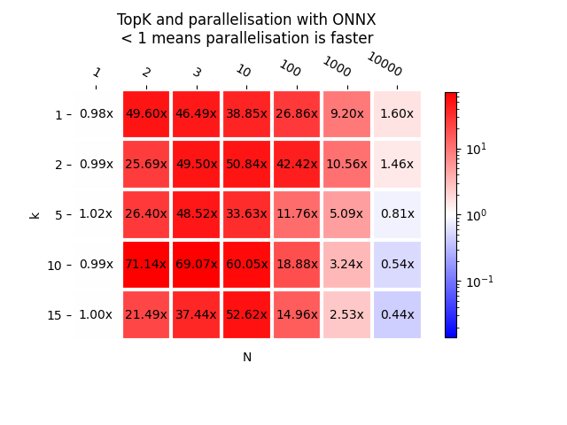
As a graph.
plot_metric(bench_onnx_para, transpose=False,
            title="TopK and parallelisation with ONNX\n< 1 means "
            "parallelisation is faster", shrink=0.75)
Out:
<AxesSubplot:title={'center':'TopK and parallelisation with ONNX\n< 1 means parallelisation is faster'}, xlabel='N', ylabel='k'>
Pretty much the same results.
onnxruntime vs mlprodict (no parallelisation)#
sess = InferenceSession(model_onnx.SerializeToString())


bench_ort = benchmark_test(
    X32, (lambda x, k: sess.run(
        None, {'X': x, 'k': numpy.array([k], dtype=numpy.int64)})),
    (lambda x, k: oinf_no_para.run(
        {'X': x, 'k': numpy.array([k], dtype=numpy.int64)})),
    N=N, K=K)
bench_ort
Out:
  0%|          | 0/5 [00:00<?, ?it/s]
 20%|##        | 1/5 [00:50<03:23, 50.79s/it]
 40%|####      | 2/5 [01:42<02:34, 51.60s/it]
 60%|######    | 3/5 [02:35<01:43, 51.95s/it]
 80%|########  | 4/5 [03:30<00:53, 53.04s/it]
100%|##########| 5/5 [04:25<00:00, 54.08s/it]
100%|##########| 5/5 [04:25<00:00, 53.19s/it]

{(1, 1): 1.2399499156868747, (2, 1): 1.2094894848183175, (3, 1): 1.2105110564726131, (10, 1): 1.19044942514807, (100, 1): 1.1083407957783988, (1000, 1): 0.9113368931400883, (10000, 1): 3.085530624873318, (1, 2): 1.2523970421376955, (2, 2): 1.2588352129887856, (3, 2): 1.260563258463255, (10, 2): 1.2399222644514638, (100, 2): 1.1154792452364959, (1000, 2): 0.9348969271371034, (10000, 2): 3.3511550574368503, (1, 5): 1.2029171752316001, (2, 5): 1.1875865586033656, (3, 5): 1.1836905404868134, (10, 5): 1.1459635885564035, (100, 5): 1.006216120685874, (1000, 5): 2.291875340616187, (10000, 5): 3.2273500464994513, (1, 10): 1.2234724125898908, (2, 10): 1.2381808356335182, (3, 10): 1.2273196255323788, (10, 10): 1.1613369045063797, (100, 10): 0.9700041883458369, (1000, 10): 3.019908951236195, (10000, 10): 3.2239363879588776, (1, 15): 1.210372412861998, (2, 15): 1.2275438077356726, (3, 15): 1.214728783284041, (10, 15): 1.1342570067644326, (100, 15): 0.9274965821838104, (1000, 15): 3.07315536998904, (10000, 15): 3.203859125109382}
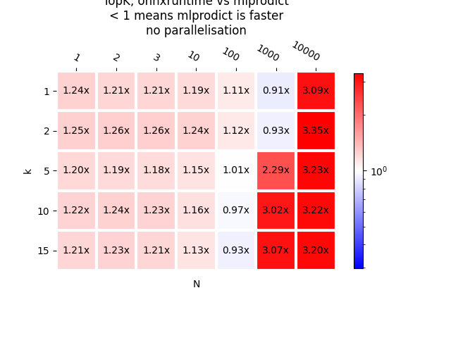
As a graph.
plot_metric(bench_ort, transpose=False,
            title="TopK, onnxruntime vs mlprodict\n< 1 means mlprodict "
            "is faster\nno parallelisation", shrink=0.75)
Out:
<AxesSubplot:title={'center':'TopK, onnxruntime vs mlprodict\n< 1 means mlprodict is faster\nno parallelisation'}, xlabel='N', ylabel='k'>
It seems the implementation of operator TopK in onnxruntime 1.1.1 can be improved.
Versions:
ort_version, mlp_version
Out:
('1.11.0', '0.8.1762')
And with parallelisation above 50 rows.
oinf_para.sequence_[0].ops_.th_para = 50
bench_ort_para = benchmark_test(
    X32, (lambda x, k: sess.run(
        None, {'X': x, 'k': numpy.array([k], dtype=numpy.int64)})),
    (lambda x, k: oinf_para.run(
        {'X': x, 'k': numpy.array([k], dtype=numpy.int64)})),
    N=N, K=K)
bench_ort_para
Out:
  0%|          | 0/5 [00:00<?, ?it/s]
 20%|##        | 1/5 [00:56<03:47, 57.00s/it]
 40%|####      | 2/5 [01:51<02:46, 55.58s/it]
 60%|######    | 3/5 [02:48<01:52, 56.19s/it]
 80%|########  | 4/5 [03:45<00:56, 56.50s/it]
100%|##########| 5/5 [04:44<00:00, 57.41s/it]
100%|##########| 5/5 [04:44<00:00, 56.90s/it]

{(1, 1): 1.2505949602987918, (2, 1): 1.2575817835047145, (3, 1): 1.2518761364734767, (10, 1): 1.2435556169333721, (100, 1): 54.17368450163326, (1000, 1): 17.33084434239648, (10000, 1): 7.8733501828184815, (1, 2): 1.2151734105527625, (2, 2): 1.2534168980600628, (3, 2): 1.251783848412169, (10, 2): 1.2366884322143938, (100, 2): 33.3121952674599, (1000, 2): 4.90139308882305, (10000, 2): 4.171299002833656, (1, 5): 1.2168394636681619, (2, 5): 1.2456791695217482, (3, 5): 1.2323706642295496, (10, 5): 1.1981445249633078, (100, 5): 27.577476020804642, (1000, 5): 9.816508210814916, (10000, 5): 2.5538622256802945, (1, 10): 1.195007625008709, (2, 10): 1.183188460079545, (3, 10): 1.1691493752968305, (10, 10): 1.1190647081525935, (100, 10): 10.066629137023765, (1000, 10): 8.67901152305891, (10000, 10): 1.7435514623457984, (1, 15): 1.2172619035593142, (2, 15): 1.233174811429135, (3, 15): 1.216972500976091, (10, 15): 1.126908399446414, (100, 15): 9.799250815552321, (1000, 15): 6.421975992523156, (10000, 15): 1.4566611547745267}
As a graph.
plot_metric(bench_ort_para, transpose=False,
            title="TopK, onnxruntime vs mlprodict\n< 1 means mlprodict "
            "is faster\nparallelisation above 50 rows", shrink=0.75)
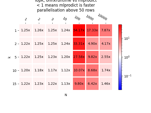
Out:
<AxesSubplot:title={'center':'TopK, onnxruntime vs mlprodict\n< 1 means mlprodict is faster\nparallelisation above 50 rows'}, xlabel='N', ylabel='k'>
- onnxruntime and mlprodict implement the same algorithm.
The only difference comes from the threshold which trigger the parallelisation. It should depend on the machine. That explains the difference in time for 100 observations.
X = numpy.array([
    [0, 1, 2, 3],
    [4, 5, 6, 7],
    [8, 9, 10, 11],
], dtype=numpy.float32)

K = numpy.array([3], dtype=numpy.int64)


node = OnnxTopK('X', K, output_names=['values', 'indices'],
                op_version=12)
onx = node.to_onnx([('X', FloatTensorType())])

py_topk = OnnxInference(onx, runtime="python_compiled")
ort_topk = InferenceSession(onx.SerializeToString())
Check the outputs.
r1 = py_topk.run({'X': X})
r1
Out:
{'values': array([[ 3.,  2.,  1.],
       [ 7.,  6.,  5.],
       [11., 10.,  9.]], dtype=float32), 'indices': array([[3, 2, 1],
       [3, 2, 1],
       [3, 2, 1]])}
r2 = ort_topk.run(None, {'X': X})
r2
Out:
[array([[ 3.,  2.,  1.],
       [ 7.,  6.,  5.],
       [11., 10.,  9.]], dtype=float32), array([[3, 2, 1],
       [3, 2, 1],
       [3, 2, 1]], dtype=int64)]
Some figures.
bs = []
bs.append(measure_time(lambda: py_topk.run({'X': X}),
                       context=globals(), div_by_number=True))
bs[-1]['c'] = 'py'
bs[-1]
Out:
{'average': 6.372089684009551e-05, 'deviation': 5.553969884520887e-07, 'min_exec': 6.322313100099564e-05, 'max_exec': 6.524350494146346e-05, 'repeat': 10, 'number': 50, 'ttime': 0.0006372089684009551, 'context_size': 2272, 'c': 'py'}
bs.append(measure_time(lambda: ort_topk.run(None, {'X': X}),
                       context=globals(), div_by_number=True))
bs[-1]['c'] = 'or'
bs[-1]
Out:
{'average': 6.829253584146499e-05, 'deviation': 6.741774447923558e-07, 'min_exec': 6.774332374334335e-05, 'max_exec': 7.021646946668625e-05, 'repeat': 10, 'number': 50, 'ttime': 0.00068292535841465, 'context_size': 2272, 'c': 'or'}
X = numpy.random.randn(10000, 100).astype(numpy.float32)


bs.append(measure_time(lambda: py_topk.run({'X': X}),
                       context=globals(), div_by_number=True))
bs[-1]['c'] = 'py-100'
bs[-1]
Out:
{'average': 0.010219269327819348, 'deviation': 0.00018311647805134725, 'min_exec': 0.009838960394263267, 'max_exec': 0.010480948910117149, 'repeat': 10, 'number': 50, 'ttime': 0.10219269327819347, 'context_size': 2272, 'c': 'py-100'}
bs.append(measure_time(lambda: ort_topk.run(None, {'X': X}),
                       context=globals(), div_by_number=True))
bs[-1]['c'] = 'ort-100'
bs[-1]
Out:
{'average': 0.0026605716310441493, 'deviation': 1.4536568251660117e-05, 'min_exec': 0.0026473639160394667, 'max_exec': 0.0026886112987995147, 'repeat': 10, 'number': 50, 'ttime': 0.026605716310441493, 'context_size': 2272, 'c': 'ort-100'}
df = DataFrame(bs)
df
Total running time of the script: ( 19 minutes 48.620 seconds)