Train, convert and predict with ONNX Runtime

This example demonstrates an end to end scenario starting with the training of a machine learned model to its use in its converted from.

Train a logistic regression

The first step consists in retrieving the iris datset.

from sklearn.datasets import load_iris
from sklearn.linear_model import LogisticRegression
from sklearn.model_selection import train_test_split

iris = load_iris()
X, y = iris.data, iris.target
X_train, X_test, y_train, y_test = train_test_split(X, y)

Then we fit a model.

clr = LogisticRegression()
clr.fit(X_train, y_train)

/home/xadupre/miniconda3/lib/python3.10/site-packages/sklearn/linear_model/_logistic.py:458: ConvergenceWarning: lbfgs failed to converge (status=1):
STOP: TOTAL NO. of ITERATIONS REACHED LIMIT.

Increase the number of iterations (max_iter) or scale the data as shown in:
    https://scikit-learn.org/stable/modules/preprocessing.html
Please also refer to the documentation for alternative solver options:
    https://scikit-learn.org/stable/modules/linear_model.html#logistic-regression
  n_iter_i = _check_optimize_result(

LogisticRegression()

In a Jupyter environment, please rerun this cell to show the HTML representation or trust the notebook.
On GitHub, the HTML representation is unable to render, please try loading this page with nbviewer.org.

We compute the prediction on the test set and we show the confusion matrix.

from sklearn.metrics import confusion_matrix

pred = clr.predict(X_test)
print(confusion_matrix(y_test, pred))

[[12  0  0]
 [ 0 11  1]
 [ 0  0 14]]

Conversion to ONNX format

We use module sklearn-onnx to convert the model into ONNX format.

from skl2onnx import convert_sklearn
from skl2onnx.common.data_types import FloatTensorType

initial_type = [("float_input", FloatTensorType([None, 4]))]
onx = convert_sklearn(clr, initial_types=initial_type)
with open("logreg_iris.onnx", "wb") as f:
    f.write(onx.SerializeToString())

We load the model with ONNX Runtime and look at its input and output.

import onnxruntime as rt

sess = rt.InferenceSession("logreg_iris.onnx", providers=rt.get_available_providers())

print("input name='{}' and shape={}".format(sess.get_inputs()[0].name, sess.get_inputs()[0].shape))
print("output name='{}' and shape={}".format(sess.get_outputs()[0].name, sess.get_outputs()[0].shape))

input name='float_input' and shape=[None, 4]
output name='output_label' and shape=[None]

We compute the predictions.

input_name = sess.get_inputs()[0].name
label_name = sess.get_outputs()[0].name

import numpy

pred_onx = sess.run([label_name], {input_name: X_test.astype(numpy.float32)})[0]
print(confusion_matrix(pred, pred_onx))

[[12  0  0]
 [ 0 11  0]
 [ 0  0 15]]

The prediction are perfectly identical.

Probabilities

Probabilities are needed to compute other relevant metrics such as the ROC Curve. Let’s see how to get them first with scikit-learn.

prob_sklearn = clr.predict_proba(X_test)
print(prob_sklearn[:3])

[[1.23548038e-04 1.39888269e-01 8.59988183e-01]
 [1.35220009e-04 1.68499463e-01 8.31365317e-01]
 [9.66261602e-01 3.37375214e-02 8.76185849e-07]]

And then with ONNX Runtime. The probabilies appear to be

prob_name = sess.get_outputs()[1].name
prob_rt = sess.run([prob_name], {input_name: X_test.astype(numpy.float32)})[0]

import pprint

pprint.pprint(prob_rt[0:3])

[{0: 0.00012354807404335588, 1: 0.13988836109638214, 2: 0.8599880337715149},
 {0: 0.00013521959772333503, 1: 0.16849936544895172, 2: 0.8313654661178589},
 {0: 0.9662615656852722, 1: 0.03373752906918526, 2: 8.761855383454531e-07}]

Let’s benchmark.

from timeit import Timer


def speed(inst, number=5, repeat=10):
    timer = Timer(inst, globals=globals())
    raw = numpy.array(timer.repeat(repeat, number=number))
    ave = raw.sum() / len(raw) / number
    mi, ma = raw.min() / number, raw.max() / number
    print("Average %1.3g min=%1.3g max=%1.3g" % (ave, mi, ma))
    return ave


print("Execution time for clr.predict")
speed("clr.predict(X_test)")

print("Execution time for ONNX Runtime")
speed("sess.run([label_name], {input_name: X_test.astype(numpy.float32)})[0]")

Execution time for clr.predict
Average 9.63e-05 min=9.02e-05 max=0.000132
Execution time for ONNX Runtime
Average 3.14e-05 min=2.98e-05 max=4.36e-05

3.140551852993667e-05

Let’s benchmark a scenario similar to what a webservice experiences: the model has to do one prediction at a time as opposed to a batch of prediction.

def loop(X_test, fct, n=None):
    nrow = X_test.shape[0]
    if n is None:
        n = nrow
    for i in range(0, n):
        im = i % nrow
        fct(X_test[im : im + 1])


print("Execution time for clr.predict")
speed("loop(X_test, clr.predict, 50)")


def sess_predict(x):
    return sess.run([label_name], {input_name: x.astype(numpy.float32)})[0]


print("Execution time for sess_predict")
speed("loop(X_test, sess_predict, 50)")

Execution time for clr.predict
Average 0.00402 min=0.00393 max=0.00413
Execution time for sess_predict
Average 0.000849 min=0.000829 max=0.000875

0.0008492533001117408

Let’s do the same for the probabilities.

print("Execution time for predict_proba")
speed("loop(X_test, clr.predict_proba, 50)")


def sess_predict_proba(x):
    return sess.run([prob_name], {input_name: x.astype(numpy.float32)})[0]


print("Execution time for sess_predict_proba")
speed("loop(X_test, sess_predict_proba, 50)")

Execution time for predict_proba
Average 0.0054 min=0.00529 max=0.00571
Execution time for sess_predict_proba
Average 0.00121 min=0.00116 max=0.00132

0.0012056639592628927

This second comparison is better as ONNX Runtime, in this experience, computes the label and the probabilities in every case.

Benchmark with RandomForest

We first train and save a model in ONNX format.

from sklearn.ensemble import RandomForestClassifier

rf = RandomForestClassifier(n_estimators=10)
rf.fit(X_train, y_train)

initial_type = [("float_input", FloatTensorType([1, 4]))]
onx = convert_sklearn(rf, initial_types=initial_type)
with open("rf_iris.onnx", "wb") as f:
    f.write(onx.SerializeToString())

We compare.

sess = rt.InferenceSession("rf_iris.onnx", providers=rt.get_available_providers())


def sess_predict_proba_rf(x):
    return sess.run([prob_name], {input_name: x.astype(numpy.float32)})[0]


print("Execution time for predict_proba")
speed("loop(X_test, rf.predict_proba, 50)")

print("Execution time for sess_predict_proba")
speed("loop(X_test, sess_predict_proba_rf, 50)")

Execution time for predict_proba
Average 0.0644 min=0.0609 max=0.072
Execution time for sess_predict_proba
Average 0.0011 min=0.00108 max=0.00115

0.0011018258426338434

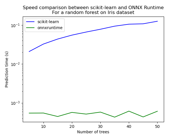
Let’s see with different number of trees.

measures = []

for n_trees in range(5, 51, 5):
    print(n_trees)
    rf = RandomForestClassifier(n_estimators=n_trees)
    rf.fit(X_train, y_train)
    initial_type = [("float_input", FloatTensorType([1, 4]))]
    onx = convert_sklearn(rf, initial_types=initial_type)
    with open("rf_iris_%d.onnx" % n_trees, "wb") as f:
        f.write(onx.SerializeToString())
    sess = rt.InferenceSession("rf_iris_%d.onnx" % n_trees, providers=rt.get_available_providers())

    def sess_predict_proba_loop(x):
        return sess.run([prob_name], {input_name: x.astype(numpy.float32)})[0]

    tsk = speed("loop(X_test, rf.predict_proba, 25)", number=5, repeat=4)
    trt = speed("loop(X_test, sess_predict_proba_loop, 25)", number=5, repeat=4)
    measures.append({"n_trees": n_trees, "sklearn": tsk, "rt": trt})

from pandas import DataFrame

df = DataFrame(measures)
ax = df.plot(x="n_trees", y="sklearn", label="scikit-learn", c="blue", logy=True)
df.plot(x="n_trees", y="rt", label="onnxruntime", ax=ax, c="green", logy=True)
ax.set_xlabel("Number of trees")
ax.set_ylabel("Prediction time (s)")
ax.set_title("Speed comparison between scikit-learn and ONNX Runtime\nFor a random forest on Iris dataset")
ax.legend()

5
Average 0.021 min=0.0207 max=0.0212
Average 0.000548 min=0.000522 max=0.000601
10
Average 0.0326 min=0.031 max=0.0335
Average 0.00055 min=0.000527 max=0.00058
15
Average 0.0438 min=0.0427 max=0.0457
Average 0.000448 min=0.000395 max=0.000568
20
Average 0.0552 min=0.0545 max=0.056
Average 0.000571 min=0.000544 max=0.00063
25
Average 0.0663 min=0.0634 max=0.0698
Average 0.000517 min=0.000407 max=0.000777
30
Average 0.0783 min=0.0777 max=0.0794
Average 0.000582 min=0.000563 max=0.000603
35
Average 0.094 min=0.0925 max=0.0955
Average 0.000431 min=0.000416 max=0.00046
40
Average 0.106 min=0.103 max=0.108
Average 0.000616 min=0.000586 max=0.000649
45
Average 0.108 min=0.107 max=0.111
Average 0.000437 min=0.000419 max=0.000475
50
Average 0.126 min=0.118 max=0.131
Average 0.000612 min=0.000587 max=0.000665

<matplotlib.legend.Legend object at 0x7f2f5ce9cfa0>