Profile the runtime memory of a model with the event log#

When a RuntimeContext runs a model with event logging enabled, it records a RuntimeEvent for every tensor map mutation and every node dispatch. Attaching a SimpleRawBufferAllocator to the context makes each event additionally carry the allocator’s live footprint (allocated_bytes, the total size of every buffer alive at that moment) and its peak footprint (peak_bytes, the maximum ever reached). Together with the wall-clock duration_ns of each node this turns the event log into a per-node time-and-memory profile.

This example:

builds a small graph that materialises two intermediate activations (Mul then Add) so the allocator’s live memory grows and shrinks as nodes run,
attaches a SimpleRawBufferAllocator to a ReferenceEvaluator and runs it with events_enabled=True and release_intermediates=True,
prints RuntimeEvent.summary() for every recorded event — a one-line recap including the live and peak memory,
isolates the per-node run_node events to read the duration and the allocator memory observed right after each node,
renders a compact table of the memory profile.

from __future__ import annotations

import numpy as np

from onnx_light.onnx_lib import parser
from onnx_light.onnx.reference import ReferenceEvaluator
from onnx_light.onnx_py._onnxpykernels import runtime as _runtime
from onnx_light.tools import pretty_onnx

Build a small ONNX model#

The graph computes w = (x * two) + x. Both z = x * two and w = z + x are intermediate activations the runtime has to hold in memory while the graph runs.

model = parser.parse_model(
    '<ir_version: 10, opset_import: ["" : 18]>'
    "agraph (float[N] x) => (float[N] w) "
    "<float two = {2.0}>"
    "{"
    "  z = Mul(x, two)"
    "  w = Add(z, x)"
    "}"
)
print(pretty_onnx(model))

opset: domain='' version=18
graph: name='agraph'
input: float[N] x
init: float[] two
0: Mul(x, two) -> z
1: Add(z, x) -> w
output: float[N] w

Attach an allocator and run with event logging#

SimpleRawBufferAllocator is a fixed-capacity pool: capacity is the maximum number of buffers that may be alive at the same time (a generous upper bound is fine — empty slots are cheap). Passing it to ReferenceEvaluator routes the runtime’s buffer storage through it, so every recorded event reports the live and peak memory. release_intermediates=True frees each intermediate as soon as its last consumer has run, which is exactly what makes the live footprint go down again in the log.

allocator = _runtime.SimpleRawBufferAllocator(64)
sess = ReferenceEvaluator(
    model, events_enabled=True, release_intermediates=True, allocator=allocator
)

x = np.arange(1024, dtype=np.float32)
(w,) = sess.run(None, {"x": x})
print(f"w[:4] = {w[:4]}")

w[:4] = [0. 3. 6. 9.]

Read the event log#

RuntimeEvent.summary() renders each event as a single line. The mem= field is the allocator’s live footprint right after the action and peak= is the largest footprint reached so far.

events = sess.events()
print(f"Recorded {len(events)} event(s):")
for ev in events:
    print(f"  {ev.summary()}")

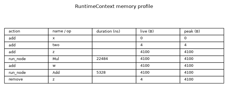
Recorded 7 event(s):
  [add/input] 'x' mem=0B peak=0B
  [add/initializer] 'two' mem=4B peak=4B
  [add/intermediate] 'z' node#0 mem=4100B peak=4100B
  [run_node/unknown] ai.onnx::Mul(x, two) node#0 took 22484ns executor#4/2 mem=4100B peak=4100B
  [add/intermediate] 'w' node#1 mem=4100B peak=4100B
  [run_node/unknown] ai.onnx::Add(z, x) node#1 took 5328ns executor#4/2 mem=4100B peak=4100B
  [remove/unknown] 'z' mem=4B peak=4100B

Isolate the per-node memory profile#

The run_node events summarise the dispatch of each node: its op_type, the duration_ns it took and the allocator memory observed right after it ran. Filtering the log by action recovers just those entries.

run_nodes = [ev for ev in events if ev.action == _runtime.RuntimeEventAction.kRunNode]
print("Per-node time and memory profile:")
for ev in run_nodes:
    d = ev.as_dict()
    print(
        f"  {d['op_type']:<8s} took {d['duration_ns']:>8d} ns  "
        f"live={d['allocated_bytes']:>6d} B  peak={d['peak_bytes']:>6d} B"
    )

Per-node time and memory profile:
  Mul      took    22484 ns  live=  4100 B  peak=  4100 B
  Add      took     5328 ns  live=  4100 B  peak=  4100 B

The allocator also exposes the peak directly#

The same peak is available on the allocator object itself, independently of the event log.

print(f"Allocator peak footprint: {allocator.peak_allocated_size} bytes")

Allocator peak footprint: 4100 bytes

Render the memory profile as a table#

A simple matplotlib figure doubles as the sphinx-gallery thumbnail and a compact recap of the recorded events, showing the live and peak memory next to each action.

import matplotlib.pyplot as plt  # noqa: E402

rows = []
for ev in events:
    d = ev.as_dict()
    label = d["op_type"] if d["action"] == "run_node" else d["name"]
    rows.append(
        [
            d["action"],
            label,
            str(d["duration_ns"]) if d["action"] == "run_node" else "",
            str(d["allocated_bytes"]),
            str(d["peak_bytes"]),
        ]
    )

fig, ax = plt.subplots(figsize=(8, 1.6 + 0.3 * len(rows)))
ax.set_axis_off()
table = ax.table(
    cellText=rows,
    colLabels=["action", "name / op", "duration (ns)", "live (B)", "peak (B)"],
    loc="center",
    cellLoc="left",
    colLoc="left",
)
table.auto_set_font_size(False)
table.set_fontsize(9)
table.scale(1.0, 1.3)
ax.set_title("RuntimeContext memory profile")
fig.tight_layout()
fig.savefig("plot_runtime_memory.png")