Gradient and training loop for linear regression

This example shows how to use onnx_light.onnx_core.gradient to:

1. Build a simple linear-regression forward model as a list of ONNX nodes.

2. Compute its gradient with respect to the trainable parameters (weights and bias) using gradient_of_nodes().

3. Run a plain gradient-descent training loop entirely in NumPy — the gradient FunctionProto tells which ONNX operations to execute backward, but the numerical evaluation is done by hand here to keep the example self-contained.

The model is y = X @ W + b where X is the feature matrix (shape [N, F]), W is the weight vector (shape [F, 1]), and b is a scalar bias. The loss is the mean-squared error (MSE) L = mean((y_pred - y_true) ** 2).

Analytical gradients

For the MSE loss L and prediction y_pred = X @ W + b:

• dL/dW = (2/N) * X.T @ (y_pred - y_true)

• dL/db = (2/N) * sum(y_pred - y_true)

The gradient FunctionProto produced by gradient_of_nodes() captures exactly this backward computation as a reusable ONNX function.

from __future__ import annotations

import numpy as np

Build the forward graph

The forward pass y = X @ W + b is expressed as two ONNX nodes: a MatMul followed by an Add.

from onnx_light.onnx_proto._helper import make_node  # noqa: E402

forward_nodes = [
    make_node("MatMul", ["X", "W"], ["mm"]),
    make_node("Add", ["mm", "b"], ["y_pred"]),
]

print("Forward nodes:")
for n in forward_nodes:
    print(f"  {n.op_type}({list(n.input)}) -> {list(n.output)}")

Forward nodes:
  MatMul(['X', 'W']) -> ['mm']
  Add(['mm', 'b']) -> ['y_pred']

Compute the gradient FunctionProto

gradient_of_nodes() performs reverse-mode automatic differentiation over the forward nodes and returns a FunctionProto that encodes the backward computation.

• xs — parameters to differentiate with respect to (W and b).

• y — the scalar (or tensor) output whose gradient is propagated back.

• zs — non-differentiable inputs (the feature matrix X).

from onnx_light.onnx_core.gradient import gradient_of_nodes  # noqa: E402

grad_fn = gradient_of_nodes(
    nodes=forward_nodes,
    inputs=["X", "W", "b"],
    initializers=[],
    xs=["W", "b"],
    y="y_pred",
    zs=["X"],
)

print("\nGradient FunctionProto:")
print(f"  inputs  = {list(grad_fn.input)}")
print(f"  outputs = {list(grad_fn.output)}")
print(f"  nodes   = {[str(n.op_type) for n in grad_fn.node]}")

Gradient FunctionProto:
  inputs  = ['W', 'b', 'X', 'dy']
  outputs = ['grad_W', 'grad_b']
  nodes   = ['Transpose', 'MatMul', 'Transpose', 'MatMul', 'Identity', 'Identity']

Training loop with NumPy

The gradient FunctionProto describes the backward pass symbolically. To actually train, we evaluate the analytical gradients in NumPy. A real training framework would execute the FunctionProto directly; here we use the NumPy equivalents to keep the example dependency-free.

# Reproducible random seed
rng = np.random.default_rng(42)

# --- Synthetic dataset ---
N, F = 200, 4  # 200 samples, 4 features
W_true = rng.standard_normal((F, 1)).astype(np.float32)
b_true = np.float32(1.5)
X_data = rng.standard_normal((N, F)).astype(np.float32)
y_data = X_data @ W_true + b_true + 0.05 * rng.standard_normal((N, 1)).astype(np.float32)

# --- Initialize parameters ---
W = rng.standard_normal((F, 1)).astype(np.float32) * 0.1
b = np.float32(0.0)

learning_rate = 0.05
n_epochs = 60
loss_history: list[float] = []

for _epoch in range(n_epochs):
    # Forward pass
    y_pred = X_data @ W + b  # shape [N, 1]
    residual = y_pred - y_data  # shape [N, 1]
    loss = float(np.mean(residual**2))
    loss_history.append(loss)

    # Backward pass (MSE loss: dL/dy_pred = 2 * residual / N)
    dy = (2.0 / N) * residual  # shape [N, 1]

    # Gradient of y_pred = X @ W + b
    #   dL/dW = X.T @ dy          (shape [F, 1])
    #   dL/db = sum(dy)            (scalar)
    grad_W = X_data.T @ dy
    grad_b = float(np.sum(dy))

    # Gradient-descent update
    W -= learning_rate * grad_W
    b -= learning_rate * grad_b

print(f"\nTraining summary (lr={learning_rate}, epochs={n_epochs}):")
print(f"  Initial loss : {loss_history[0]:.4f}")
print(f"  Final   loss : {loss_history[-1]:.6f}")
print(f"  Learned W    : {W.ravel()}")
print(f"  True    W    : {W_true.ravel()}")
print(f"  Learned b    : {b:.4f}  (true: {b_true:.4f})")

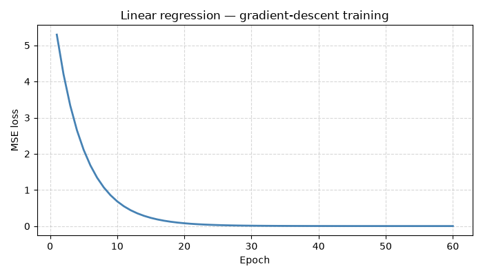
Training summary (lr=0.05, epochs=60):
  Initial loss : 5.2952
  Final   loss : 0.002554
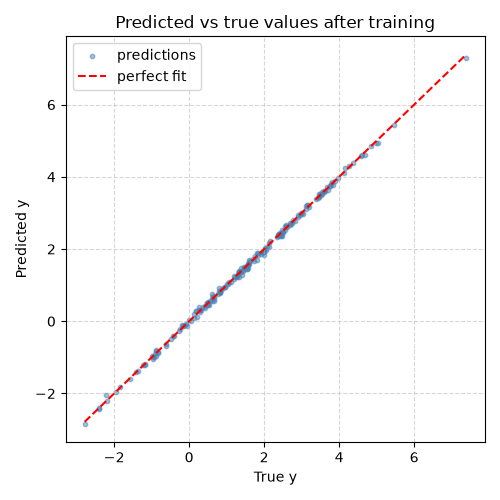
  Learned W    : [ 0.30281866 -1.0434434   0.75531673  0.93419707]
  True    W    : [ 0.3047171 -1.0399841  0.7504512  0.9405647]
  Learned b    : 1.4949  (true: 1.5000)

Plot — loss curve

import matplotlib.pyplot as plt  # noqa: E402

fig, ax = plt.subplots(figsize=(7, 4))
ax.plot(range(1, n_epochs + 1), loss_history, linewidth=2, color="steelblue")
ax.set_xlabel("Epoch")
ax.set_ylabel("MSE loss")
ax.set_title("Linear regression — gradient-descent training")
ax.grid(True, linestyle="--", alpha=0.5)
fig.tight_layout()
fig.savefig("plot_gradient_linear_regression.png")

Plot — predicted vs true values

y_final = X_data @ W + b
fig2, ax2 = plt.subplots(figsize=(5, 5))
ax2.scatter(y_data, y_final, s=10, alpha=0.5, color="steelblue", label="predictions")
lims = [float(y_data.min()), float(y_data.max())]
ax2.plot(lims, lims, "r--", linewidth=1.5, label="perfect fit")
ax2.set_xlabel("True y")
ax2.set_ylabel("Predicted y")
ax2.set_title("Predicted vs true values after training")
ax2.legend()
ax2.grid(True, linestyle="--", alpha=0.5)
fig2.tight_layout()
fig2.savefig("plot_gradient_linear_regression_scatter.png")

Related examples

Example last updated

Date:

2026-08-21