ComputeContext memory expressions#

ComputeContext reports, for each node, how much memory is already live before execution, how much extra output allocation is still needed, and the resulting total. When input shapes are symbolic, these quantities stay symbolic as well.

This example shows how to:

Build a small graph with one symbolic dimension N.
Run every analysis at once with ComputeContext.compute().
Print a table with the symbolic memory expressions for every node.
Evaluate total_bytes for a few concrete values of N and plot the resulting curves.

from __future__ import annotations

import matplotlib.pyplot as plt
import onnx_light.onnx as onnxl
import onnx_light.onnx.defs as defs
import onnx_light.onnx.helper as oh
from onnx_light.tools import pretty_onnx
from onnx_light.onnx_core.expressions import evaluate_expression
from onnx_light.onnx_core.shape_inference import (
    ComputeContext,
    NODE_MEMORY_ALREADY_ALLOCATED_BYTES_KEY,
    NODE_MEMORY_INPUTS_KEY,
    NODE_MEMORY_INITIALIZERS_KEY,
    NODE_MEMORY_INTERMEDIATES_KEY,
    NODE_MEMORY_OUTPUT_ALLOCATION_BYTES_KEY,
    NODE_MEMORY_OUTPUTS_KEY,
    NODE_MEMORY_TOTAL_BYTES_KEY,
)

# Built-in operator schemas must be registered before shape inference.
defs.register_onnx_operator_set_schema()

Build a graph with one symbolic dimension#

The graph keeps the rank fixed but leaves the leading dimension symbolic:

X : float[N, 4]
W : float[4, 4]
M = MatMul(X, W)     -> float[N, 4]
C = Concat(M, X)     -> float[2*N, 4]
S = Shape(C)         -> int64[2]
A = Abs(C)           -> float[2*N, 4]
Z = Reshape(A, S)    -> float[2*N, 4]

W contributes constant initializer memory, Concat turns the symbolic leading dimension into 2*N, S is tagged as a shape tensor, and the last two nodes can reuse their input buffers in place. The memory table therefore mixes constant terms, symbolic terms, and zero-allocation steps.

model = oh.make_model(
    oh.make_graph(
        [
            oh.make_node("MatMul", ["X", "W"], ["M"]),
            oh.make_node("Concat", ["M", "X"], ["C"], axis=0),
            oh.make_node("Shape", ["C"], ["S"]),
            oh.make_node("Abs", ["C"], ["A"]),
            oh.make_node("Reshape", ["A", "S"], ["Z"]),
        ],
        "compute_context_memory_demo",
        inputs=[oh.make_tensor_value_info("X", onnxl.TensorProto.FLOAT, ["N", 4])],
        outputs=[oh.make_tensor_value_info("Z", onnxl.TensorProto.FLOAT, None)],
        initializer=[
            oh.make_tensor(
                "W",
                onnxl.TensorProto.FLOAT,
                [4, 4],
                [1.0, 0.0, 0.0, 0.0, 0.0, 1.0, 0.0, 0.0, 0.0, 0.0, 1.0, 0.0, 0.0, 0.0, 0.0, 1.0],
            )
        ],
    ),
    opset_imports=[oh.make_opsetid("", 18)],
    ir_version=8,
)

print(pretty_onnx(model))

opset: domain='' version=18
graph: name='compute_context_memory_demo'
input: float[N,4] X
init: float[4,4] W
0: MatMul(X, W) -> M
1: Concat(M, X) -> C
2: Shape(C) -> S
3: Abs(C) -> A
4: Reshape(A, S) -> Z
output: float[] Z

Run every analysis at once#

ComputeContext.compute() chains shape inference, value/node tagging, in-place reuse (with release-after and shape-tag classification) and per-node peak memory, keeping every result alive inside the context. The symbolic shapes it infers, the semantic shape tags and the reuse opportunities all feed the per-node memory buckets. ComputeContext.write_to_model() then pushes the inferred shapes and annotations back into the model.

compute_context = ComputeContext()
compute_context.compute(model)
compute_context.write_to_model(model)
memory_profiles = compute_context.memory


MemoryScalar = int | str


def evaluate_memory_scalar(value: MemoryScalar, assignment: dict[str, int]) -> int:
    """Evaluates *value* under *assignment*.

    Returns:
        The evaluated integer result.
    """

    if isinstance(value, int):
        return value
    return evaluate_expression(value, assignment)


def format_bucket(bucket: dict[str, MemoryScalar]) -> str:
    """Formats one tagged memory bucket.

    Returns:
        A stable string rendering of the bucket.
    """

    if not bucket:
        return "-"
    parts = []
    for tag, value in sorted(bucket.items(), key=lambda item: (item[0] != "", item[0])):
        label = "untagged" if tag == "" else tag
        parts.append(f"{label}={value}")
    return ", ".join(parts)

Symbolic per-node memory table#

The table below shows the symbolic profile computed for each node:

already_allocated is the live memory at node entry,
output_allocation is the fresh allocation still required for outputs,
total is their sum.

The source buckets make it easy to see which bytes come from live inputs, initializers, intermediates, or newly allocated outputs.

rows = []
for node_index, node in enumerate(model.graph.node):
    profile = memory_profiles[node_index]
    rows.append(
        [
            str(node_index),
            node.op_type,
            str(profile[NODE_MEMORY_ALREADY_ALLOCATED_BYTES_KEY]),
            str(profile[NODE_MEMORY_OUTPUT_ALLOCATION_BYTES_KEY]),
            format_bucket(profile[NODE_MEMORY_INPUTS_KEY]),
            format_bucket(profile[NODE_MEMORY_INITIALIZERS_KEY]),
            format_bucket(profile[NODE_MEMORY_INTERMEDIATES_KEY]),
            format_bucket(profile[NODE_MEMORY_OUTPUTS_KEY]),
            str(profile[NODE_MEMORY_TOTAL_BYTES_KEY]),
        ]
    )

headers = [
    "node",
    "op",
    "already_allocated",
    "output_allocation",
    "inputs",
    "initializers",
    "intermediates",
    "outputs",
    "total",
]
col_widths = [len(h) for h in headers]
for row in rows:
    for i, cell in enumerate(row):
        if len(cell) > col_widths[i]:
            col_widths[i] = len(cell)
separator = "  " + "  ".join("-" * w for w in col_widths)
header_line = "  " + "  ".join(h.ljust(col_widths[i]) for i, h in enumerate(headers))
print("Symbolic ComputeContext.memory table:")
print(separator)
print(header_line)
print(separator)
for row in rows:
    print("  " + "  ".join(cell.ljust(col_widths[i]) for i, cell in enumerate(row)))
print(separator)

Symbolic ComputeContext.memory table:
  ----  -------  -----------------  -----------------  -----------  ------------  ---------------------  -----------  -------
  node  op       already_allocated  output_allocation  inputs       initializers  intermediates          outputs      total
  ----  -------  -----------------  -----------------  -----------  ------------  ---------------------  -----------  -------
  0     MatMul   16*N+64            16*N               weight=16*N  weight=64     -                      weight=16*N  32*N+64
  1     Concat   32*N+64            32*N               weight=16*N  weight=64     weight=16*N            weight=32*N  64*N+64
  2     Shape    48*N+64            16                 weight=16*N  weight=64     weight=32*N            shape=16     48*N+80
  3     Abs      48*N+80            0                  weight=16*N  weight=64     shape=16, weight=32*N  -            48*N+80
  4     Reshape  48*N+80            0                  weight=16*N  weight=64     shape=16, weight=32*N  -            48*N+80
  ----  -------  -----------------  -----------------  -----------  ------------  ---------------------  -----------  -------

Per-node peak scratch memory#

ComputeContext.compute() also estimates the extra scratch memory each operator needs on top of its inputs and outputs. Operators without a registered peak-memory function (or whose relevant shapes stay symbolic) report 0.

print("\nPer-node peak scratch memory (bytes):")
for node_index, node in enumerate(model.graph.node):
    peak = compute_context.node_peak_memory(node_index)
    print(f"  node{node_index} {node.op_type:>8}: {peak}")

Per-node peak scratch memory (bytes):
  node0   MatMul: 0
  node1   Concat: 0
  node2    Shape: 0
  node3      Abs: 0
  node4  Reshape: 0

Evaluate the symbolic expressions#

Once concrete values are chosen for N, the symbolic totals become plain integers. Each line below evaluates the same node-wise total_bytes curve under a different assignment.

ASSIGNMENTS = [{"N": 1}, {"N": 8}, {"N": 32}, {"N": 128}]
node_indices = list(range(len(memory_profiles)))

print("\nEvaluated total_bytes per node:")
print(f"  {'N':>6} " + " ".join(f"node{i:>2}" for i in node_indices))
evaluated_totals: dict[int, list[int]] = {}
for assignment in ASSIGNMENTS:
    n_value = assignment["N"]
    totals = [
        evaluate_memory_scalar(profile[NODE_MEMORY_TOTAL_BYTES_KEY], assignment)
        for profile in memory_profiles
    ]
    evaluated_totals[n_value] = totals
    print(f"  {n_value:>6} " + " ".join(f"{value:>6}" for value in totals))

fig, ax = plt.subplots(figsize=(8, 4.5))
for n_value, totals in evaluated_totals.items():
    ax.plot(node_indices, totals, marker="o", linewidth=2, label=f"N={n_value}")

ax.set_xticks(node_indices)
ax.set_xticklabels([f"{i}:{node.op_type}" for i, node in enumerate(model.graph.node)])
ax.set_xlabel("node index")
ax.set_ylabel("total bytes")
ax.set_title("Evaluated ComputeContext.total_bytes")
ax.grid(True, alpha=0.3)
ax.legend()
fig.tight_layout()
fig.savefig("plot_compute_context_memory.png")

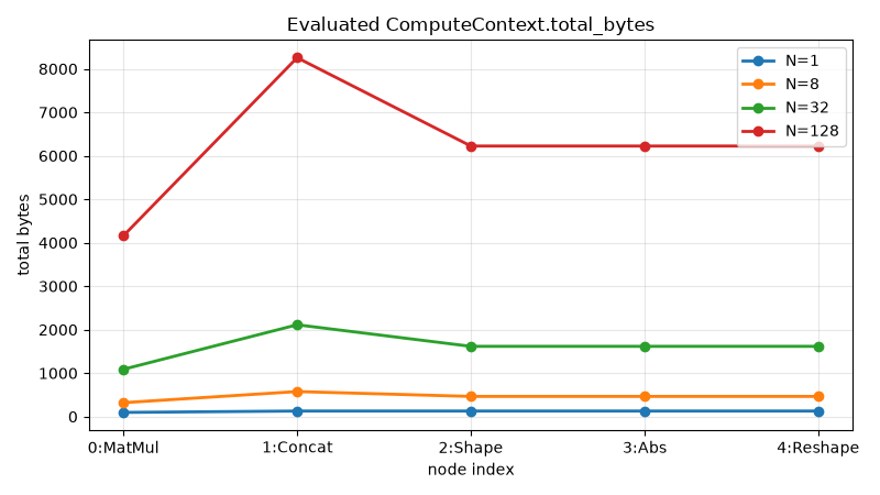
Evaluated total_bytes per node:
       N node 0 node 1 node 2 node 3 node 4
       1     96    128    128    128    128
       8    320    576    464    464    464
      32   1088   2112   1616   1616   1616
     128   4160   8256   6224   6224   6224

Total running time of the script: (0 minutes 0.117 seconds)

Download Jupyter notebook: plot_compute_context_memory.ipynb

Download Python source code: plot_compute_context_memory.py

Download zipped: plot_compute_context_memory.zip

Related examples