Processor performance profile: memory, compute, and Roofline

This example calls onnx_light_cpu.benchmark_processor_performance() – the single public entry point produced by the processor performance profile roadmap – and renders its returned ProcessorPerformanceProfile end to end: topology, working-set sizes, warnings, a compact measurement table, memory bandwidth/latency plots, an arithmetic throughput plot, and a Roofline chart.

It does not re-implement any measurement: every number plotted below comes straight from the profile returned by that one call. Every reported number is an effective, working-set measurement taken on this exact host – never a hardware maximum, a physical link rate, or a guaranteed peak (see the roadmap document linked above for the full measurement contract).

The two participant policies answer different questions. single runs one worker (pinned to the requested logical processor when affinity is available); physical runs one worker per process-visible physical core, deliberately excluding extra simultaneous-multithreading siblings. The latter therefore reports aggregate throughput across physical cores, not throughput from one core.

Setup

UNITTEST_GOING=1 shrinks the measurement (fewer repeats, shorter duration, a smaller memory budget) so the example still runs quickly as a unit test while exercising every public result path: both thread policies, latency, an explicit affinity, and every element type this host can supply.

import argparse
import json
import os
import platform
from pathlib import Path

import matplotlib.pyplot as plt
import numpy as np

from onnx_light_cpu import ExplicitAffinity, benchmark_processor_performance


def _processor_name():
    cpuinfo = Path("/proc/cpuinfo")
    if cpuinfo.exists():
        for line in cpuinfo.read_text(encoding="utf-8").splitlines():
            key, separator, value = line.partition(":")
            if separator and key.strip() == "model name":
                return value.strip()
    return platform.processor() or "unknown"


unit_test_going = os.environ.get("UNITTEST_GOING", "0") in ("1", "true", "True")

# ``--repeats``/``--minimum-duration-ms`` let the measurement be lengthened
# (e.g. to steady the noisy ``physical`` policy on a busy or high-core-count
# host) without touching the source. ``parse_known_args`` ignores unrelated
# arguments injected by pytest/sphinx-gallery when this file runs as a test
# or a documentation example.
parser = argparse.ArgumentParser(description=__doc__)
parser.add_argument(
    "--repeats",
    type=int,
    default=2 if unit_test_going else 12,
    help="number of measurement repeats per (dtype, policy) combination",
)
parser.add_argument(
    "--minimum-duration-ms",
    type=float,
    default=1.0 if unit_test_going else 40.0,
    help="minimum wall-clock duration, in milliseconds, of a single measurement sample",
)
args, _ = parser.parse_known_args()

print(
    f"benchmark parameters: repeats={args.repeats} minimum_duration_ms={args.minimum_duration_ms}"
)

profile = benchmark_processor_performance(
    thread_policies=("single", "physical"),
    repeats=args.repeats,
    minimum_duration_ms=args.minimum_duration_ms,
    memory_budget_bytes=(8 * 1024 * 1024) if unit_test_going else (128 * 1024 * 1024),
    include_latency=True,
    explicit_single_affinity=ExplicitAffinity(0, 0),
)

benchmark parameters: repeats=12 minimum_duration_ms=40.0

Topology, selected affinities, and working-set sizes

Everything below is read from profile.topology and profile.memory / profile.compute – no separate measurement is taken here.

A cache descriptor’s sharing_thread_count is the number of logical processors that share that cache instance: one means private to one logical processor, while a larger value means shared by that many logical processors. It does not mean that every cache at a given level has one global instance.

topology = profile.topology
print(f"processor={_processor_name()}")
print(f"platform={profile.metadata.platform} compiler={profile.metadata.compiler}")
print(f"timer={profile.metadata.timer_name} schema_version={profile.metadata.schema_version}")
print(
    f"logical_threads={topology.logical_thread_count} "
    f"physical_cores={topology.physical_core_count} "
    f"performance_cores={topology.performance_core_count} "
    f"efficiency_cores={topology.efficiency_core_count} "
    f"cache_topology_detected={topology.cache_topology_detected}"
)
for cache in topology.caches:
    print(
        f"  L{cache.level} {cache.kind:<9} size={cache.size_bytes:>10} bytes "
        f"line={cache.line_size_bytes:>3} sharing_threads={cache.sharing_thread_count:>3} "
        f"confidence={cache.confidence}"
    )

print("\nselected affinities and working-set sizes (memory levels):")
for level, policies in profile.memory.items():
    for policy, entry in policies.items():
        reference = entry.read or entry.write or entry.copy or entry.read_modify_write
        if reference is None:
            continue
        print(
            f"  {level:<3} {policy:<8} participants={reference.participant_count:<2} "
            f"affinity_pinned={reference.affinity_pinned!s:<5} "
            f"working_set={reference.working_set_bytes:>10} bytes"
        )

if profile.warnings:
    print("\nwarnings:")
    for warning in profile.warnings:
        print(f"  - {warning}")

processor=AMD EPYC 9V74 80-Core Processor
platform=linux compiler=gcc
timer=std::chrono::steady_clock schema_version=2
logical_threads=4 physical_cores=2 performance_cores=2 efficiency_cores=0 cache_topology_detected=True
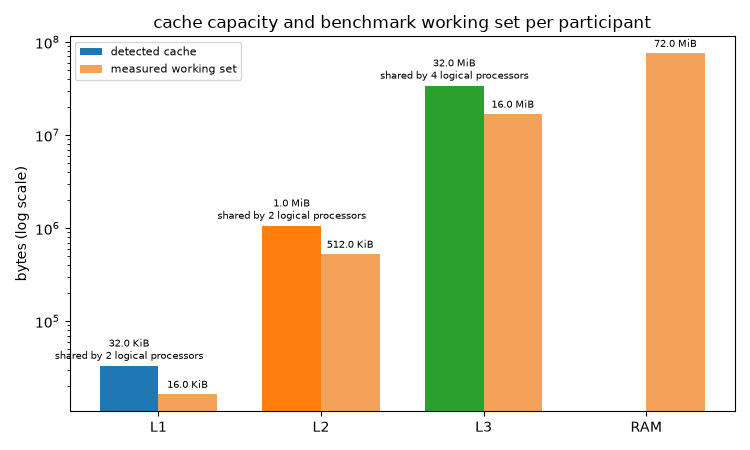
  L1 data      size=     32768 bytes line= 64 sharing_threads=  2 confidence=detected
  L1 instruction size=     32768 bytes line= 64 sharing_threads=  2 confidence=detected
  L2 unified   size=   1048576 bytes line= 64 sharing_threads=  2 confidence=detected
  L3 unified   size=  33554432 bytes line= 64 sharing_threads=  4 confidence=detected

selected affinities and working-set sizes (memory levels):
  L1  single   participants=1  affinity_pinned=True  working_set=     16384 bytes
  L1  physical participants=2  affinity_pinned=True  working_set=     16384 bytes
  L2  single   participants=1  affinity_pinned=True  working_set=    524288 bytes
  L2  physical participants=2  affinity_pinned=True  working_set=    524288 bytes
  L3  single   participants=1  affinity_pinned=True  working_set=  16777216 bytes
  L3  physical participants=2  affinity_pinned=True  working_set=  16777216 bytes
  RAM single   participants=1  affinity_pinned=True  working_set=  75497472 bytes

warnings:
  - memory RAM read (physical): working set unavailable for the requested memory level
  - memory RAM write (physical): working set unavailable for the requested memory level
  - memory RAM copy (physical): working set unavailable for the requested memory level
  - memory RAM read_modify_write (physical): working set unavailable for the requested memory level
  - memory RAM latency (physical): working set unavailable for the requested memory level
  - compute float16 (single): no compiled and runtime-detected native arithmetic path for this element type
  - compute float16 (physical): no compiled and runtime-detected native arithmetic path for this element type

Plot 1: cache hierarchy and measured working sets

The detected cache capacities and the actual per-participant working sets are different quantities, so both are shown. L1/L2/L3 measurements choose working sets inside the named cache level; RAM chooses one larger than the last-level cache. Cache annotations state whether each selected cache descriptor is private or how many logical processors share it. RAM has no detected capacity: its bar is only the working set used by the benchmark.

def _format_bytes(value):
    if value >= 1024**2:
        return f"{value / 1024**2:.1f} MiB"
    return f"{value / 1024:.1f} KiB"


levels = list(profile.memory.keys())
cache_by_level = {}
for cache in topology.caches:
    if cache.kind not in ("data", "unified"):
        continue
    level = f"L{cache.level}"
    if level not in cache_by_level or cache.size_bytes > cache_by_level[level].size_bytes:
        cache_by_level[level] = cache

working_sets = {}
for level, policies in profile.memory.items():
    entry = policies.get("single") or next(iter(policies.values()))
    reference = entry.read or entry.write or entry.copy or entry.read_modify_write
    if reference is not None:
        working_sets[level] = reference.working_set_bytes

fig_hierarchy, ax_hierarchy = plt.subplots(1, 1, figsize=(7.5, 4.5))
x = np.arange(len(levels))
width = 0.36
for i, level in enumerate(levels):
    cache = cache_by_level.get(level)
    if cache is not None:
        ax_hierarchy.bar(
            i - width / 2,
            cache.size_bytes,
            width,
            label="detected cache" if i == 0 else "",
        )
        sharing = (
            "private to 1 logical processor"
            if cache.sharing_thread_count == 1
            else f"shared by {cache.sharing_thread_count} logical processors"
        )
        ax_hierarchy.annotate(
            f"{_format_bytes(cache.size_bytes)}\n{sharing}",
            (i - width / 2, cache.size_bytes),
            xytext=(0, 3),
            textcoords="offset points",
            ha="center",
            va="bottom",
            fontsize=7,
        )
    if level in working_sets:
        value = working_sets[level]
        ax_hierarchy.bar(
            i + width / 2,
            value,
            width,
            label="measured working set" if i == 0 else "",
            color="#f4a259",
        )
        ax_hierarchy.annotate(
            _format_bytes(value),
            (i + width / 2, value),
            xytext=(0, 3),
            textcoords="offset points",
            ha="center",
            va="bottom",
            fontsize=7,
        )
ax_hierarchy.set_yscale("log")
ax_hierarchy.set_xticks(x)
ax_hierarchy.set_xticklabels(levels)
ax_hierarchy.set_ylabel("bytes (log scale)")
ax_hierarchy.set_title("cache capacity and benchmark working set per participant")
ax_hierarchy.legend(fontsize=8)
fig_hierarchy.tight_layout()
fig_hierarchy.savefig("plot_processor_performance_hierarchy.png")

How to read this figure

One group of bars per memory level (L1, L2, L3, RAM), on a logarithmic byte scale. The two bars measure different things and are not two estimates of the same quantity:

• detected cache (left bar) is the capacity of the cache instance reported by the CPU topology for that level (cache.size_bytes). Its annotation adds the sharing scope read from sharing_thread_count: either private to one logical processor, or shared by N logical processors. It is a hardware property, not something measured here.

• measured working set (right bar) is the amount of data one benchmark participant deliberately walks during the measurement (working_set_bytes). It is a benchmark input size chosen so the traffic lands in the intended level, not a second estimate of the cache capacity.

“Per participant” matters because each worker owns disjoint storage: with the physical policy, the total footprint is this working set multiplied by the number of participants.

The two values differ on purpose. For L1/L2/L3 the working set is chosen comfortably below the detected capacity so the data stays resident in that level once warmed (leaving room for the other data structures and for a cache shared with sibling threads). For RAM the working set is chosen above the last-level cache so the traffic really reaches memory; RAM has no detected capacity, so only the working-set bar is drawn. A missing left bar therefore means “no cache descriptor at this level”, never “capacity zero”.

Compact measurement table

One line per available (level/policy) bandwidth+latency measurement and per (element type/policy) compute measurement. Values are the median of the raw samples retained in the profile; all figures are effective measurements on this host, not a hardware specification.

print("\nmemory bandwidth (effective, median of raw samples):")
print(f"  {'level':<4} {'policy':<8} {'read GB/s':>10} {'write GB/s':>11} {'copy GB/s':>10}")
for level, policies in profile.memory.items():
    for policy, entry in policies.items():
        read = entry.read.median_gbps if entry.read else float("nan")
        write = entry.write.median_gbps if entry.write else float("nan")
        copy = entry.copy.median_gbps if entry.copy else float("nan")
        print(f"  {level:<4} {policy:<8} {read:>10.2f} {write:>11.2f} {copy:>10.2f}")

print("\ncompute throughput (effective, median of raw samples, GOP/s):")
compute_policies = [
    p for p in ("single", "physical") if any(p in v for v in profile.compute.values())
]
header = f"  {'dtype':<9} {'impl':<10}" + "".join(f"{p:>12}" for p in compute_policies)
print(header)
for element_type, policies in profile.compute.items():
    implementation_name = next(iter(policies.values())).implementation_name
    row = f"  {element_type:<9} {implementation_name:<10}"
    for policy in compute_policies:
        entry = policies.get(policy)
        row += f"{entry.median_gops:>12.2f}" if entry else f"{'--':>12}"
    print(row)

memory bandwidth (effective, median of raw samples):
  level policy    read GB/s  write GB/s  copy GB/s
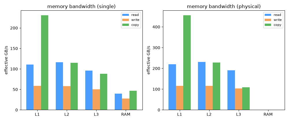
  L1   single       110.73       58.61     231.05
  L1   physical     219.92      115.76     456.08
  L2   single       116.23       58.16     115.04
  L2   physical     231.40      115.41     228.01
  L3   single        95.70       50.11      88.01
  L3   physical     190.51      102.84     108.90
  RAM  single        39.82       27.70      46.45

compute throughput (effective, median of raw samples, GOP/s):
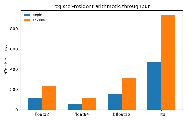
  dtype     impl            single    physical
  float32   AVX-512         117.43      233.82
  float64   AVX-512          58.71      116.08
  bfloat16  AVX-512         156.54      311.35
  int8      AVX-512         469.63      933.43

Plot 2: bandwidth by memory level

Each recorded sample times repeated sequential aligned streams after warmup: loads for read, cached stores for write, and one source plus one destination for copy. Useful bytes are divided by elapsed monotonic wall-clock time, then the plot uses the median across recorded samples. Each participant owns disjoint storage; physical values are aggregate bandwidth.

policies_order = [
    p for p in ("single", "physical") if any(p in profile.memory[lv] for lv in levels)
]
modes = ("read", "write", "copy")
mode_colors = {"read": "#4a9eff", "write": "#f4a259", "copy": "#5cb85c"}

fig, axes = plt.subplots(
    1, max(1, len(policies_order)), figsize=(5 * max(1, len(policies_order)), 4.2), squeeze=False
)
for ax, policy in zip(axes[0], policies_order, strict=True):
    x = np.arange(len(levels))
    width = 0.25
    for i, mode in enumerate(modes):
        values = []
        for level in levels:
            entry = profile.memory[level].get(policy)
            measurement = getattr(entry, mode, None) if entry is not None else None
            values.append(measurement.median_gbps if measurement is not None else 0.0)
        ax.bar(x + (i - 1) * width, values, width, label=mode, color=mode_colors[mode])
    ax.set_xticks(x)
    ax.set_xticklabels(levels)
    ax.set_ylabel("effective GB/s")
    ax.set_title(f"memory bandwidth ({policy})")
    ax.legend(fontsize=8)
fig.tight_layout()
fig.savefig("plot_processor_performance_bandwidth.png")

How to read this figure

One panel per thread policy, one group of bars per memory level, three series per group:

• read streams the working set with loads only;

• write streams it with cached stores only;

• copy streams one source and one destination, so it touches twice as many bytes per element as read or write.

The vertical axis is effective GB/s: useful bytes divided by the elapsed wall-clock time of the timed region, then the median over the recorded samples (median_gbps). “Effective” means it is what this host actually delivered for that access pattern, including any hardware prefetching and coherence traffic – it is not a datasheet peak, and it can legitimately be lower than a theoretical bus rate. Higher is better.

The two panels are not comparable one-to-one. The single panel is the throughput of a single worker (pinned when affinity is available). The physical panel is aggregate throughput summed over one worker per process-visible physical core, each on its own disjoint buffer; it typically scales with core count in the private caches (L1, L2) and flattens in L3/RAM where the resource is shared. A zero-height bar means that traffic mode was unavailable for that level/policy; profile.warnings printed above says why.

Plot 3: aggregate read bandwidth scaling by core count

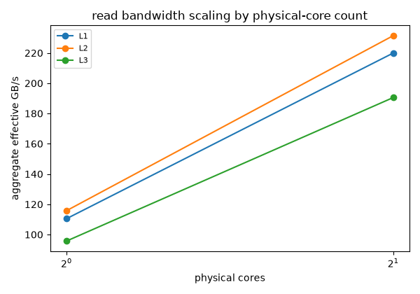
The physical-core measurement also records intermediate powers of two, making cache and memory-bandwidth saturation visible instead of reporting only the one-core and all-core endpoints.

fig_scaling, ax_scaling = plt.subplots(1, 1, figsize=(6, 4.2))
for level in ("L1", "L2", "L3"):
    entry = profile.memory.get(level, {}).get("physical")
    if entry is None or not entry.read_scaling:
        continue
    ax_scaling.plot(
        [point.participant_count for point in entry.read_scaling],
        [point.median_gbps for point in entry.read_scaling],
        marker="o",
        label=level,
    )
ax_scaling.set_xscale("log", base=2)
ax_scaling.set_xlabel("physical cores")
ax_scaling.set_ylabel("aggregate effective GB/s")
ax_scaling.set_title("read bandwidth scaling by physical-core count")
ax_scaling.legend(fontsize=8)
fig_scaling.tight_layout()
fig_scaling.savefig("plot_processor_performance_bandwidth_scaling.png")

How to read this figure

One curve per cache level, taken from entry.read_scaling of the physical policy. The horizontal axis (log base 2) is the number of concurrent participants, i.e. physical cores actually running the read stream, from one up to the process-visible physical core count; the vertical axis is the aggregate effective read bandwidth of all those participants combined, each on its own disjoint working set of the size shown in the first figure.

Read the shape, not only the endpoint. A curve that keeps following a straight line of slope one on this log axis means the level scales: each added core contributes roughly the same bandwidth, so the resource is private. A curve that bends and flattens marks saturation: past that participant count the shared resource (a shared last-level cache, the ring or mesh interconnect, the memory controllers) is the limit, and adding cores buys nothing. The knee is the practical parallelism budget for a kernel whose traffic lives at that level. A missing curve means no scaling series was recorded for that level.

Plot 4: dependent-load latency by memory level

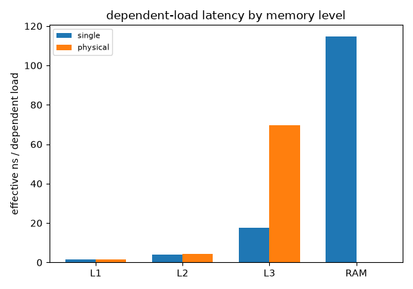
Latency uses a randomized single-cycle pointer permutation built before timing. Every load determines the address of the next, preventing overlap; the plotted value is the median nanoseconds per dependent load.

fig_lat, ax_lat = plt.subplots(1, 1, figsize=(6, 4.2))
x = np.arange(len(levels))
width = 0.35
for i, policy in enumerate(policies_order):
    values = []
    for level in levels:
        entry = profile.memory[level].get(policy)
        values.append(
            entry.latency.median_ns_per_load if entry is not None and entry.latency else 0.0
        )
    ax_lat.bar(x + (i - 0.5) * width, values, width, label=policy)
ax_lat.set_xticks(x)
ax_lat.set_xticklabels(levels)
ax_lat.set_ylabel("effective ns / dependent load")
ax_lat.set_title("dependent-load latency by memory level")
ax_lat.legend(fontsize=8)
fig_lat.tight_layout()
fig_lat.savefig("plot_processor_performance_latency.png")

How to read this figure

One group of bars per memory level, one bar per thread policy. The value is latency.median_ns_per_load: the median nanoseconds spent per dependent load. Unlike the bandwidth figure, lower is better here.

The measurement is a pointer chase. Before timing, the working set is arranged as a random cyclic permutation of pointers – one chain visiting every element exactly once before closing on itself; the timed loop then follows that chain, so the address of load n+1 is the value returned by load n. Neither the out-of-order engine nor the hardware prefetcher can overlap the accesses or guess the next address, which is why the result is a serialized latency – the full time to resolve one access at that level – and not a throughput divided by a queue depth.

Values grow with the level (a few nanoseconds in L1, tens of nanoseconds in RAM), and the jumps between groups show where each level of the hierarchy starts. Comparing the two policies shows contention: physical runs one independent chain per core, so a value visibly above the single one means concurrent traffic is slowing individual accesses down. A zero-height bar means no latency measurement was available for that level/policy.

Plot 5: arithmetic throughput by element type and thread policy

Small native kernels keep independent operands and accumulators in registers, so this measures arithmetic rather than memory traffic. Operations are divided by elapsed monotonic wall-clock time and medians are plotted; a fused multiply-add counts as two floating-point operations.

element_types = list(profile.compute.keys())
fig_compute, ax_compute = plt.subplots(1, 1, figsize=(6.5, 4.2))
x = np.arange(len(element_types))
width = 0.35
for i, policy in enumerate(policies_order):
    values = [
        (
            profile.compute[element_type][policy].median_gops
            if policy in profile.compute[element_type]
            else 0.0
        )
        for element_type in element_types
    ]
    ax_compute.bar(x + (i - 0.5) * width, values, width, label=policy)
ax_compute.set_xticks(x)
ax_compute.set_xticklabels(element_types)
ax_compute.set_ylabel("effective GOP/s")
ax_compute.set_title("register-resident arithmetic throughput")
ax_compute.legend(fontsize=8)
fig_compute.tight_layout()
fig_compute.savefig("plot_processor_performance_compute.png")

How to read this figure

One group of bars per element type actually available on this host (the keys of profile.compute, e.g. float32, float64, and the reduced precisions when supported), one bar per thread policy. The table printed above names, for each element type, the implementation_name – the kernel variant the dispatcher selected, which is what makes wider vector types look faster.

The vertical axis is effective GOP/s: the number of arithmetic operations issued divided by the elapsed wall-clock time, median over the recorded samples (median_gops). Higher is better. The counting convention is the usual one: a fused multiply-add counts as two operations (one multiply, one add), so an FMA-based kernel reports twice the operation count of a plain-add kernel doing the same number of instructions.

The kernel keeps independent operands and accumulators in registers, so the figure isolates arithmetic capability from memory traffic: it is a compute ceiling for this host, again measured rather than derived from a clock frequency times a vector width. single is one worker; physical is the aggregate over one worker per physical core, so it is expected to be several times higher, and the ratio between the two bars shows how well arithmetic scales before shared front-end or power limits kick in. A missing bar means that element type was not measured for that policy.

Plot 6: Roofline

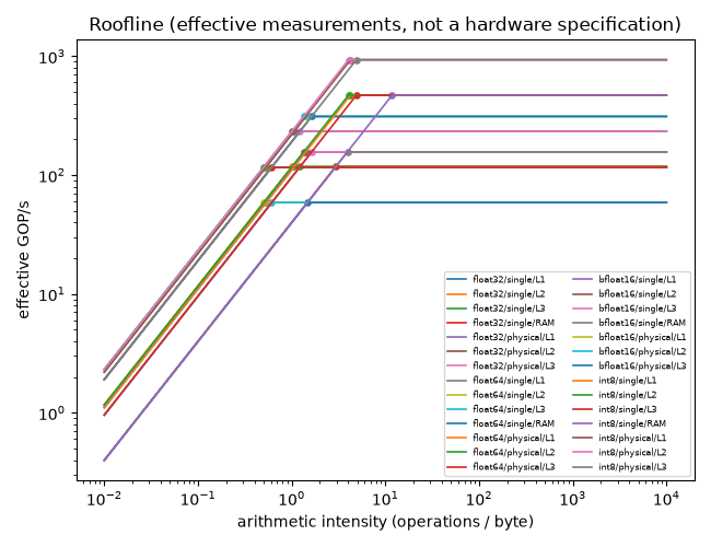
Every point below is read from profile.roofline: a horizontal ceiling at the measured compute throughput for one element type/policy, a diagonal ceiling derived from the measured read bandwidth of one memory level, and their crossover arithmetic intensity. These are derived quantities that still link back to the exact compute and memory measurements they were computed from – not an idealized hardware Roofline.

fig_roof, ax_roof = plt.subplots(1, 1, figsize=(6.5, 5))
intensity = np.logspace(-2, 4, 200)
for element_type, per_policy in profile.roofline.items():
    for policy, per_level in per_policy.items():
        for level, point in per_level.items():
            memory_bound = point.memory_read_gbps * intensity
            roofline_curve = np.minimum(memory_bound, point.compute_gops)
            ax_roof.plot(
                intensity,
                roofline_curve,
                label=f"{element_type}/{policy}/{level}",
                linewidth=1.2,
            )
            ax_roof.scatter(
                [point.arithmetic_intensity_crossover],
                [point.compute_gops],
                marker="o",
                s=14,
            )

ax_roof.set_xscale("log")
ax_roof.set_yscale("log")
ax_roof.set_xlabel("arithmetic intensity (operations / byte)")
ax_roof.set_ylabel("effective GOP/s")
ax_roof.set_title("Roofline (effective measurements, not a hardware specification)")
ax_roof.legend(fontsize=6, ncol=2)
fig_roof.tight_layout()
fig_roof.savefig("plot_processor_performance_roofline.png")

plt.show()

How to read this figure

Both axes are logarithmic. The horizontal axis is arithmetic intensity: how many arithmetic operations a kernel performs per byte it moves from the given memory level. A kernel that reads a lot and computes little sits on the left; a kernel that reuses data heavily in registers and caches sits on the right.

Each curve is one element type / policy / level combination from profile.roofline and has two parts:

• the diagonal, memory_read_gbps * intensity, is the memory ceiling: at that intensity, the read bandwidth measured for that level physically cannot feed more operations per second;

• the plateau, compute_gops, is the compute ceiling: the arithmetic throughput measured for that element type and policy in the previous figure.

The attainable rate is the lower of the two, so the curve is their minimum. The marker sits at arithmetic_intensity_crossover, where the two ceilings meet. Left of it a kernel is memory bound – the fix is fewer bytes (blocking, fusion, a smaller element type), not faster arithmetic. Right of it, a kernel is compute bound – the fix is better vectorization or more cores.

Both ceilings come from the measurements taken in this run, not from published hardware peaks, so a kernel plotted against these curves is compared to what this host actually delivered under this benchmark’s access patterns.

Serialization

to_dict() gives a stable, versioned JSON-compatible representation of the whole profile (metadata, topology, memory, compute, roofline, and warnings), suitable for archiving alongside a run or feeding a future optimal-transport GEMM tile-placement cost model.

serialized = profile.to_dict()
assert serialized["metadata"]["schema_version"] == profile.metadata.schema_version
print(f"\nserialized profile keys: {sorted(serialized.keys())}")
print(f"serialized JSON size: {len(json.dumps(serialized))} bytes")

serialized profile keys: ['compute', 'memory', 'metadata', 'roofline', 'topology', 'warnings']
serialized JSON size: 33559 bytes