Train a linear regression with forward backward

This example rewrites Train a linear regression with onnxruntime-training with another optimizer OrtGradientForwardBackwardOptimizer. This optimizer relies on class TrainingAgent from onnxruntime-training. In this case, the user does not have to modify the graph to compute the error. The optimizer builds another graph which returns the gradient of every weights assuming the gradient on the output is known. Finally, the optimizer adds the gradients to the weights. To summarize, it starts from the following graph:

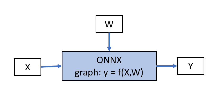
Class OrtGradientForwardBackwardOptimizer builds other ONNX graph to implement a gradient descent algorithm:

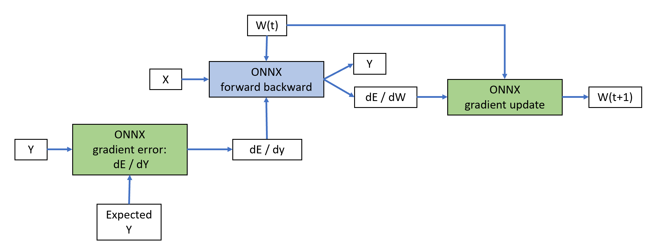
The blue node is built by class TrainingAgent (from onnxruntime-training). The green nodes are added by class OrtGradientForwardBackwardOptimizer. This implementation relies on ONNX to do the computation but it could be replaced by any other framework such as pytorch. This design gives more freedom to the user to implement his own training algorithm.

A simple linear regression with scikit-learn

from pprint import pprint
import numpy
from pandas import DataFrame
from onnxruntime import get_device
from sklearn.datasets import make_regression
from sklearn.model_selection import train_test_split
from sklearn.neural_network import MLPRegressor
from mlprodict.onnx_conv import to_onnx
from onnxcustom.plotting.plotting_onnx import plot_onnxs
from onnxcustom.utils.orttraining_helper import get_train_initializer
from onnxcustom.training.optimizers_partial import (
    OrtGradientForwardBackwardOptimizer)

X, y = make_regression(n_features=2, bias=2)
X = X.astype(numpy.float32)
y = y.astype(numpy.float32)
X_train, X_test, y_train, y_test = train_test_split(X, y)

We use a sklearn.neural_network.MLPRegressor.

lr = MLPRegressor(hidden_layer_sizes=tuple(),
                  activation='identity', max_iter=50,
                  batch_size=10, solver='sgd',
                  alpha=0, learning_rate_init=1e-2,
                  n_iter_no_change=200,
                  momentum=0, nesterovs_momentum=False)
lr.fit(X, y)
print(lr.predict(X[:5]))

Out:

/var/lib/jenkins/workspace/onnxcustom/onnxcustom_UT_39_std/_venv/lib/python3.9/site-packages/sklearn/neural_network/_multilayer_perceptron.py:692: ConvergenceWarning: Stochastic Optimizer: Maximum iterations (50) reached and the optimization hasn't converged yet.
  warnings.warn(
[-1.15975655e+02  7.97680616e-02  9.66523209e+01 -5.34809189e+01
  2.13671280e+02]

The trained coefficients are:

print("trained coefficients:", lr.coefs_, lr.intercepts_)

Out:

trained coefficients: [array([[51.089794],
       [80.767105]], dtype=float32)] [array([1.989909], dtype=float32)]

ONNX graph

Training with onnxruntime-training starts with an ONNX graph which defines the model to learn. It is obtained by simply converting the previous linear regression into ONNX.

onx = to_onnx(lr, X_train[:1].astype(numpy.float32), target_opset=15,
              black_op={'LinearRegressor'})

plot_onnxs(onx, title="Linear Regression in ONNX")

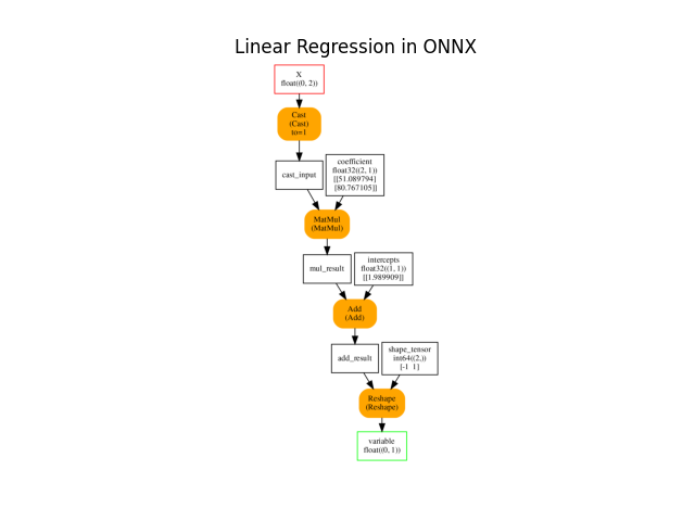
Out:

<AxesSubplot:title={'center':'Linear Regression in ONNX'}>

Weights

Every initializer is a set of weights which can be trained and a gradient will be computed for it. However an initializer used to modify a shape or to extract a subpart of a tensor does not need training. get_train_initializer removes them.

inits = get_train_initializer(onx)
weights = {k: v for k, v in inits.items() if k != "shape_tensor"}
pprint(list((k, v[0].shape) for k, v in weights.items()))

Out:

[('coefficient', (2, 1)), ('intercepts', (1, 1))]

Train on CPU or GPU if available

device = "cuda" if get_device().upper() == 'GPU' else 'cpu'
print("device=%r get_device()=%r" % (device, get_device()))

Out:

device='cpu' get_device()='CPU'

Stochastic Gradient Descent

The training logic is hidden in class OrtGradientForwardBackwardOptimizer It follows scikit-learn API (see SGDRegressor.

train_session = OrtGradientForwardBackwardOptimizer(
    onx, list(weights), device=device, verbose=1, learning_rate=1e-2,
    warm_start=False, max_iter=200, batch_size=10)

train_session.fit(X, y)

Out:

  0%|          | 0/200 [00:00<?, ?it/s]
  6%|5         | 11/200 [00:00<00:01, 109.73it/s]
 12%|#1        | 23/200 [00:00<00:01, 110.04it/s]
 18%|#7        | 35/200 [00:00<00:01, 110.24it/s]
 24%|##3       | 47/200 [00:00<00:01, 110.19it/s]
 30%|##9       | 59/200 [00:00<00:01, 110.23it/s]
 36%|###5      | 71/200 [00:00<00:01, 110.29it/s]
 42%|####1     | 83/200 [00:00<00:01, 110.24it/s]
 48%|####7     | 95/200 [00:00<00:00, 110.29it/s]
 54%|#####3    | 107/200 [00:00<00:00, 110.31it/s]
 60%|#####9    | 119/200 [00:01<00:00, 110.24it/s]
 66%|######5   | 131/200 [00:01<00:00, 110.15it/s]
 72%|#######1  | 143/200 [00:01<00:00, 110.12it/s]
 78%|#######7  | 155/200 [00:01<00:00, 110.07it/s]
 84%|########3 | 167/200 [00:01<00:00, 110.02it/s]
 90%|########9 | 179/200 [00:01<00:00, 109.97it/s]
 95%|#########5| 190/200 [00:01<00:00, 109.96it/s]
100%|##########| 200/200 [00:01<00:00, 110.09it/s]

OrtGradientForwardBackwardOptimizer(model_onnx='ir_version...', weights_to_train=['coefficient', 'intercepts'], loss_output_name='loss', max_iter=200, training_optimizer_name='SGDOptimizer', batch_size=10, learning_rate=LearningRateSGD(eta0=0.01, alpha=0.0001, power_t=0.25, learning_rate='invscaling'), value=0.0026591479484724943, device='cpu', warm_start=False, verbose=1, validation_every=20, learning_loss=SquareLearningLoss(), enable_logging=False, weight_name=None, learning_penalty=NoLearningPenalty(), exc=True)

And the trained coefficients are…

state_tensors = train_session.get_state()
pprint(["trained coefficients:", state_tensors])
print("last_losses:", train_session.train_losses_[-5:])

min_length = min(len(train_session.train_losses_), len(lr.loss_curve_))
df = DataFrame({'ort losses': train_session.train_losses_[:min_length],
                'skl losses': lr.loss_curve_[:min_length]})
df.plot(title="Train loss against iterations")

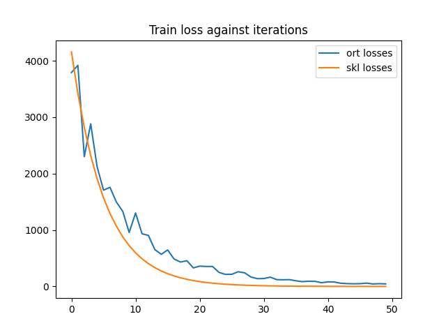
Out:

['trained coefficients:',
 [<onnxruntime.capi.onnxruntime_pybind11_state.OrtValue object at 0x7f5cde096ab0>,
  <onnxruntime.capi.onnxruntime_pybind11_state.OrtValue object at 0x7f5cde096530>]]
last_losses: [0.005264026, 0.007569605, 0.0053504906, 0.0039015156, 0.004138238]

<AxesSubplot:title={'center':'Train loss against iterations'}>

The convergence speed is almost the same.

Gradient Graph

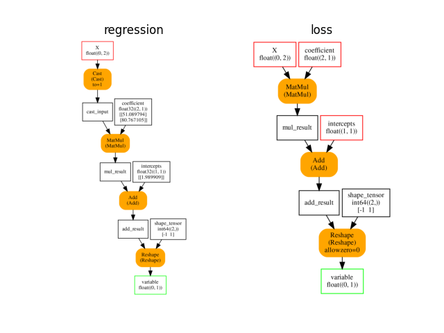
As mentioned in this introduction, the computation relies on a few more graphs than the initial graph. When the loss is needed but not the gradient, class TrainingAgent creates another graph, faster, with the trained initializers as additional inputs.

onx_loss = train_session.train_session_.cls_type_._optimized_pre_grad_model

plot_onnxs(onx, onx_loss, title=['regression', 'loss'])

Out:

array([<AxesSubplot:title={'center':'regression'}>,
       <AxesSubplot:title={'center':'loss'}>], dtype=object)

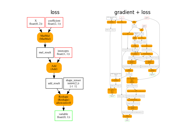
And the gradient.

onx_gradient = train_session.train_session_.cls_type_._trained_onnx

plot_onnxs(onx_loss, onx_gradient, title=['loss', 'gradient + loss'])

Out:

array([<AxesSubplot:title={'center':'loss'}>,
       <AxesSubplot:title={'center':'gradient + loss'}>], dtype=object)

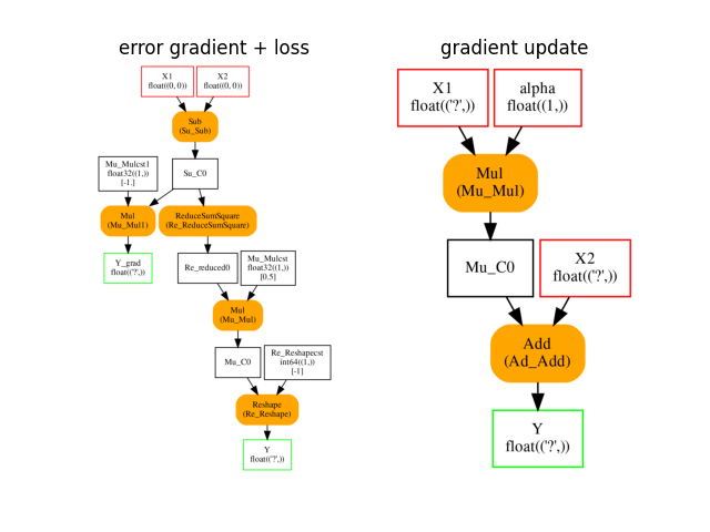
The last ONNX graphs are used to compute the gradient dE/dY and to update the weights. The first graph takes the labels and the expected labels and returns the square loss and its gradient. The second graph takes the weights and the learning rate as inputs and returns the updated weights. This graph works on tensors of any shape but with the same element type.

plot_onnxs(train_session.learning_loss.loss_grad_onnx_,
           train_session.learning_rate.axpy_onnx_,
           title=['error gradient + loss', 'gradient update'])

# import matplotlib.pyplot as plt
# plt.show()

Out:

array([<AxesSubplot:title={'center':'error gradient + loss'}>,
       <AxesSubplot:title={'center':'gradient update'}>], dtype=object)

previous

Partial Training with OrtGradientForwardBackwardOptimizer

next

Forward backward on a neural network on GPU