Save an ONNX model in the ORT flatbuffer format and compare sizes#

onnxruntime defines a flatbuffer serialization (.ort) of an ONNX model. It is typically used in size-constrained deployments because it can be memory-mapped directly into the runtime and avoids a protobuf parsing step.

onnx-light exposes the format through onnx_light.onnx.SerializeFormat, but the C++ writer for ORT_FLATBUFFERS is not implemented yet (calls raise RuntimeError). Until it lands, this example uses onnxruntime itself to produce the .ort file and then compares the on-disk sizes of the two formats as the number of nodes in the graph grows.

See html_theme.sidebar_secondary.remove for the short recipe.

import os
import shutil

import matplotlib.pyplot as plt
import numpy as np
import onnxruntime

import onnx_light.onnx as onnxl
import onnx_light.onnx.helper as oh
import onnx_light.onnx.numpy_helper as onh

Build a chain of `Gemm` nodes#

A small helper builds a model with num_nodes chained Gemm nodes (one float32 weight matrix per node) so the saved files have a non-trivial size that scales linearly with num_nodes. DIM shrinks when the example runs in the documentation build (UNITTEST_GOING=1) so the build stays cheap.

DIM = 32 if os.environ.get("UNITTEST_GOING") == "1" else 128


def build_model(num_nodes: int, dim: int = DIM) -> onnxl.ModelProto:
    """Builds an ONNX model with *num_nodes* chained ``Gemm`` nodes."""
    rng = np.random.default_rng(0)
    inputs = [oh.make_tensor_value_info("X", onnxl.TensorProto.FLOAT, [None, dim])]
    outputs = [
        oh.make_tensor_value_info(f"Y{num_nodes - 1}", onnxl.TensorProto.FLOAT, [None, dim])
    ]
    initializers = []
    nodes = []
    prev = "X"
    for i in range(num_nodes):
        w = rng.standard_normal((dim, dim)).astype(np.float32)
        w_name = f"W{i}"
        out_name = f"Y{i}"
        initializers.append(onh.from_array(w, name=w_name))
        nodes.append(oh.make_node("Gemm", [prev, w_name], [out_name], transB=1))
        prev = out_name
    graph = oh.make_graph(nodes, "demo_graph", inputs, outputs, initializer=initializers)
    return oh.make_model(graph, opset_imports=[oh.make_opsetid("", 18)], ir_version=9)

Save helpers#

The .onnx file is written by onnx_light.onnx.save(). The .ort file is produced by onnxruntime: disable graph optimizations so that the serialized graph stays structurally equivalent to the input, and set session.save_model_format=ORT so the optimized-model dump uses the flatbuffer format.

def save_as_ort(onnx_path: str, ort_path: str) -> None:
    """Saves the model at *onnx_path* as an ORT flatbuffer at *ort_path*."""
    session_options = onnxruntime.SessionOptions()
    session_options.graph_optimization_level = onnxruntime.GraphOptimizationLevel.ORT_DISABLE_ALL
    session_options.optimized_model_filepath = ort_path
    session_options.add_session_config_entry("session.save_model_format", "ORT")
    # Creating the session triggers the optimized-model dump.
    onnxruntime.InferenceSession(onnx_path, session_options, providers=["CPUExecutionProvider"])

Measure sizes for a range of node counts#

out_dir = "temp_plot_save_ort_flatbuffers"
os.makedirs(out_dir, exist_ok=True)

node_counts = [1, 2, 4, 8, 16, 32]
onnx_sizes = []
ort_sizes = []

for n in node_counts:
    model = build_model(n)
    onnx_path = os.path.join(out_dir, f"model_{n}.onnx")
    ort_path = os.path.join(out_dir, f"model_{n}.ort")
    onnxl.save(model, onnx_path)
    save_as_ort(onnx_path, ort_path)
    onnx_sizes.append(os.path.getsize(onnx_path))
    ort_sizes.append(os.path.getsize(ort_path))

print(f"{'nodes':>6} {'.onnx (KB)':>12} {'.ort (KB)':>12} {'ratio':>8}")
print("-" * 42)
for n, s_onnx, s_ort in zip(node_counts, onnx_sizes, ort_sizes):
    print(f"{n:>6} {s_onnx / 1024:>12.1f} {s_ort / 1024:>12.1f} {s_ort / s_onnx:>8.3f}")

 nodes   .onnx (KB)    .ort (KB)    ratio
------------------------------------------
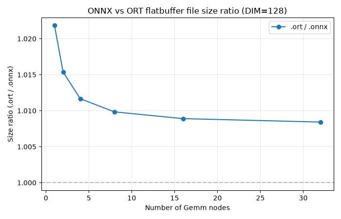
       64.1         65.5    1.022
      128.2        130.1    1.015
      256.3        259.3    1.012
      512.5        517.5    1.010
     1024.9       1034.1    1.009
     2049.9       2067.1    1.008

Plot the size ratio vs. number of nodes#

The flatbuffer payload is comparable to the protobuf one and both grow linearly with the number of weight matrices. On much larger models the .ort file is typically a bit bigger because it embeds runtime metadata; the trade-off is mmap-friendly loading without protobuf parsing. Plotting the .ort / .onnx size ratio makes the relative overhead easier to read than the raw sizes.

size_ratios = np.array(ort_sizes) / np.array(onnx_sizes)

fig, ax = plt.subplots(figsize=(7, 4.5))
ax.plot(node_counts, size_ratios, marker="o", label=".ort / .onnx")
ax.axhline(1.0, color="gray", linestyle="--", alpha=0.5)
ax.set_xlabel("Number of Gemm nodes")
ax.set_ylabel("Size ratio (.ort / .onnx)")
ax.set_title(f"ONNX vs ORT flatbuffer file size ratio (DIM={DIM})")
ax.grid(True, alpha=0.3)
ax.legend()
fig.tight_layout()

ONNX vs ORT flatbuffer file size ratio (DIM=128)

Cleanup#

shutil.rmtree(out_dir, ignore_errors=True)

Total running time of the script: (0 minutes 0.146 seconds)

Related examples

Measures loading and saving time for an ONNX model

Number of threads used to load and save ONNX models

Benchmark streaming vs in-memory alignment of external data

Gallery generated by Sphinx-Gallery